These course notes should be used to supplement what you learn in class. They are not intended to replace course lectures and discussions. You are only responsible for material covered in class; you are not responsible for any material covered in the course notes but not in class.
Overview
The setting
Dichotomous variables
Enter the indicator variable
Indicator variables in regression
Adding controls
Assumption checking
Displaying our results
Summary
Appendix
The setting
So far, aside from the first unit, we’ve been dealing exclusively with variables which are
numeric, and
(at least vaguely) continuous.
These are nicely behaved variables! They encode a great deal of information and they tend to be easy to model. When you have the choice to work with a variable on a continuous scale or a dichotomous scale (e.g., working with test scores v.s. proficiency status), we suggest sticking with the continuous variable (for lots of reasons!).
However, this isn’t always possible. We’re frequently interested in working with variables which can’t really be represented as values on a continuous numeric scale. For example, in most applications we think of gender as binary or dichotomous, respondents identify as male or female (or masculine and feminine).1 Similarly, we often wonder whether graduating from college predicts important outcomes. However a person either has or has not graduated from college; we might be able to come up with a continuous measure of educational attainment, but graduation itself has to be treated as a dichotomy.
It may not be obvious how to apply the approaches we’ve developed so far when one of the variables is categorical. This unit will develop the tools we need to do regression when one of the predictors is dichotomous. Regression with dichotomous outcomes turns out to be quite a bit different, and will not be covered in this class. However, S-052 and A-164 will both discuss logistic regression, one tool for doing regression with dichotomous outcomes, so you should totally take them!
The running example we’ll use for the class is the following: Making Caring Common (MCC), a research group interested in issues of moral development in young people, conducted a survey in multiple schools in 2014. In this analysis, we’ll be focusing on responses from a single school.
Students were asked a wide range of different questions. The survey included a scale designed to measure students’ empathic concern, i.e., their tendency to experience concern and happiness on behalf of those around them. The researchers formed a scale score by taking the average of students responses to all of these items. For example, if a student responded two to half of the items and three to the other half, he would have a scale score of 2.5. Scale scores run from one to three, and higher scores indicate more self-reported empathic concern.
Students were also asked to report how safe they felt in a number of school locations. Once again, the researchers created a scale score by taking the mean of each respondent’s answers to the nine items in the safety scale. The scale runs from one to four, and higher values indicate feeling more safe at school.
As with all self-reported measures, it’s crucial to remember that we can only measure the ways in which students present themselves on surveys. The strength of the association between self-reported empathic concern and actual empathic concern is not one we can estimate, because our only measures of empathic concern are the self-reported values. Similarly, different students might have different thresholds for what constitutes safety. There’s not really anything we can do about this, except to keep it in mind as a potential limitation to our inferences.
The research question we’d like to address is whether girls or boys report higher levels of empathic concern. We could, of course, answer that question with a t-test, but we’d like to do so using regression. We’d also like to see whether there is an association between how safe students feel in school and their reported empathy, and whether there is an association when controlling for students’ gender. This requires something more than a t-test, which can only examine the uncontrolled association between a dichotomous predictor and a continuous outcome; we can’t use a t-test to examine a controlled association.
Dichotomous variables
A dichotomous variable is a variable which has two possible values. For example, on this survey students were able to identify as either female or male. As another example, respondents might be able to identify themselves as either married or not married (on a different survey; high-schoolers would probably be weirded out by that question). When creating dichotomous variables, it’s important to use categories that are both exhaustive and mutually exclusive. Every respondent should be able to find exactly one category which describes herself. The gender dichotomy may not meet this requirement (some respondents will not identify as male or female), but probably comes reasonably close. In our running example, we’ll let the variable GENDER denote the respondent’s gender. GENDER takes on values of “Female” and “Male” in our dataset (although girl and boy might be better).
The problem with including a dichotomous variable directly in a regression should be obvious. Suppose that we want to regress empathic concern, which we’ll call EMPATHY, on gender, to determine if there’s an association between gender and empathic concern. We write out the population model as
EMPATHY_i = \beta_0+\beta_1GENDER_i+\varepsilon_i
The problem, then, is that the meaning of \beta_1GENDER_i is ill-defined. What does it mean to multiply \beta_1 by, say, ``Male’’? What we need to do is develop a technique which will allow us to represent group membership numerically in a way that makes it possible to fit and interpret a regression model.
Enter the indicator variable
The solution is a handy little hack called an indicator variable.2 We define the indicator variable MALE as follows:
That is, MALE is equal to 0 for every respondent who identifies as female, and is equal to 1 for every respondent who identifies as male. The category which is associated with a 0, in this case ``Female’’, is referred to as the reference category, for reasons that should become clearer later.
Before we consider the role of indicator variables in a regression, let’s look at how we can use them in an analysis more generally. Indicator variables turn out to be pretty nifty things. First, consider the mean of an indicator variable.
\hat{\mu}_{MALE}=\frac{\sum MALE_i}{n}
But now consider what \sum MALE_i, the sum of each respondent’s value of MALE, means. This variable takes on a value of 1 for every male respondent and a value of 0 for every female respondent, so \sum MALE_i is actually the total number of respondents who have identified themselves as male on the survey, and \sfrac{\sum MALE_i}{n} is the proportion of respondents who have identified themselves as male. If we were to take \sfrac{\sum MALE_i}{n}*100\%, that would be the percent of respondents who identified themselves as male.
The standard deviation of an indicator variable is a little less informative. In fact, the standard deviation of an indicator variable is a function of its mean. If we take \hat{\mu}_{MALE} to be the sample mean of the indicator variable (i.e. if the proportion of respondents who identify themselves as male is \hat{\mu}_{MALE}), then the standard deviation is very close to
The standard deviation is small when the proportion of male respondents is close to either 1 or 0, and is largest when the proportion is exactly equal to .5 (in which case the standard deviation is also very close to .5). The standard deviation is symmetric around the value \hat{\mu}_{MALE}=.5; the standard deviation of a sample where \hat{\mu}_{MALE}=p is identical to the standard deviation of a sample where \hat{\mu}_{MALE}=1-p. But given this, the standard deviation doesn’t really convey any information above and beyond \hat{\mu}_{MALE}, so it’s not very interesting. This is very different from the case of a numeric variable, where the mean and standard deviation are measuring very different things, and each one gives different information. We rarely report the standard deviation of an indicator variable because it is less informative than the mean, and much harder to interpret.
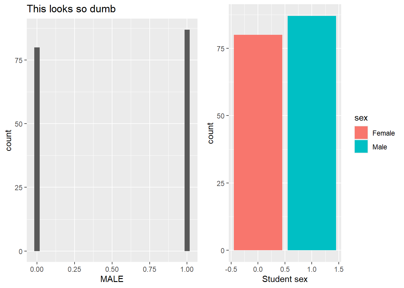
In the dataset we’re considering, the mean of MALE is .497; 92 students identified themselves as female and 91 as male. The standard deviation is almost exactly .5.
Figure 1: Two possible displays of the sample distribution of MALE. We prefer the one on the right.
Generating a sensible display of an indicator variable can take a little thought. Histograms don’t work well, because they treat the variable as though the numeric scale is actually meaningful. They tend to leave a bunch of blank space between 0 and 1. In fact, we’d suggest presenting a barplot of the original dichotomous variable instead. Figure Figure 1 shows both approaches applied in our context.
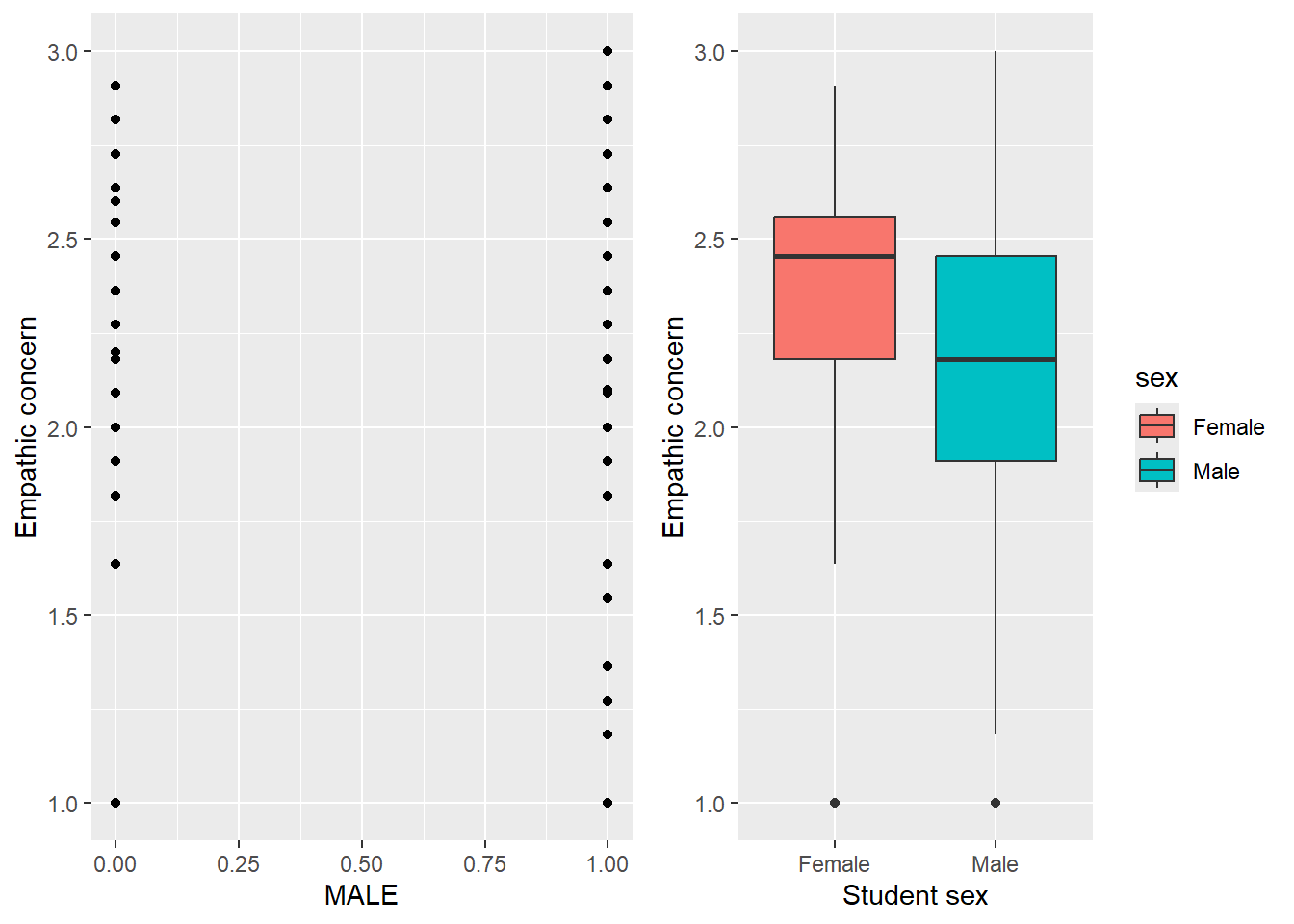
Figure 2: Two possible displays of the association between MALE and EMPATHY. We prefer the one on the right.
It’s also a little tricky to show a bivariate relationship, in our example the association between gender and empathic concern. Scatterplots don’t give much information, because all of the points have a value of MALE of exactly 0 or 1. A better option would be to show separate box-and-whisker plots or histograms for girls and boys. Figure Figure 2 shows both approaches. In our dataset, girls report mean empathy of 2.38, and boys of 2.16. To give these numbers some context, remember that the scale midpoint is 2 and the highest possible value is 3.
One interesting takeaway from this plot is that there’s a great deal more variability in reported empathy for boys than for girls. Most girls report empathy between 1.5 and 3, while most boys range from closer to 1.2 and 3. Some girls and boys report high levels, though the median is higher for girls; however, boys report levels which are much lower than girls do.
Indicator variables in regression
We’re ready now to use the indicator variable, MALE, in a regression. Before we start, let’s call the mean empathic concern score for girls \mu_{girls} and the mean empathic concern score for boys \mu_{boys} (we’re referring to population means, which you know because the \mu’s don’t have hats). The first model we’ll fit will be
To get a sense of what the parameters mean, consider that we have two sorts of respondents from the perspective of this model: girls and boys. For girls, the regression equation will look like
because girls all have a value of zero for MALE. Of course, the mean residual, \varepsilon_i, is 03 so the mean value of EMPATHY for girls, \mu_{girls}, is \beta_0. That, in fact, is the clearest interpretation of \beta_0: the population mean value of the outcome for the reference group. Notice that this means the exact same thing as our standard interpretation of an intercept, i.e., the mean or predicted value of the outcome for units with a 0 on the predictors. It’s just that a much simpler, more interpretable way to describe units who have a 0 on the MALE variable is ``girls’’.4
Now consider the situation for boys. All boys have a value of one for MALE, so for them the regression equation will look like
and the mean value of EMPATHY for boys, \mu_{boys}, is \beta_0 + \beta_1. Since \mu_{girls}=\beta_0, \beta_1 is the difference between the mean value of EMPATHY for boys and girls. Equivalently, it’s the mean difference in EMPATHY between boys and girls. This is why the group which is assigned a value of zero for the indicator variable is called the reference group; the coefficient \beta_1 can only be interpreted in reference to the mean score for girls. Once again, this is the same meaning as our typical interpretation of \beta_1. A one-unit difference in the MALE indicator variable is associated with a \beta_1 unit difference in the predicted outcome. It’s just that a one-unit difference in MALE is the difference between a boy and a girl, so a much more meaningful interpretation is that girls and boys differ, on average, in empathic concern by \beta_1 scale points.
Given this analysis, you can probably already figure out what \hat{\beta}_0 and \hat{\beta}_1 are. Girls in the sample report a mean value of empathic concern of 2.38, which means that \hat{\beta}_0=2.38. Boys in the sample report a value of 2.16, so \hat{\beta}_1 = 2.16-2.38 = -0.22. The fact that \hat{\beta}_1 is negative means that boys report lower mean empathy than girls, not that boys report negative mean empathy; the scale only goes to 1, so there’s no way to have negative empathic concern. The fitted equation is
\hat{EMPATHY}_i = 2.38 - 0.22MALE.
\hat{\beta}_1 is statistically significant (p<.001), so we conclude that girls self-report higher levels of empathy than boys in the population.
You may have noticed that in this case we were able to ``fit’’ the regression model by hand just by observing the mean values of empathic concern for girls and boys in the sample. Indicator variables tend to be easy to work with. However, Stata treats them exactly like any other predictor when it fits the model. Internally, Stata is doing the exact same matrix manipulation as it would with any other predictor. Unit 8 discusses this in more detail (or it’s supposed to; I may fail to get to it. Let me know if I forgot to).
Adding controls
You might remember another technique we used to determine whether members of different groups had the same mean in the population: the t-test. In fact, regression on an indicator variable is identical to a two-sample t-test with pooled variances (the assumption that the variances in the two groups are equal in the population, which you’ll recognize as the assumption of homoscedasticity). So regression is able to do the work of a t-test for us.5
But regression can do a lot more than a t-test, because regression also gives us the ability to add controls to the model. That’s what we’re going to do now.
We’re going to fit a series of models, to continue to build intuition around how regression works. First, we’ll regress SAFETY on MALE, then we’ll regress EMPATHY on SAFETY, and finally we’ll regress EMAPTHY on both MALE and SAFTEY. Notice that at no point do we regress MALE (the dichotomy) on any other variables. This is because regressing dichotomous outcomes on predictors takes special models (remember, S-052 and A-164 will both introduce techniques to handle dichotomous outcomes).
The first fit gives us
\hat{SAFETY}_i = 3.04 + 0.22MALE_i.
This tells us that, on average, boys feel safer than girls, by about 0.22 points on a scale from one to four. Girls report an average sense of safety of 3.04.
The second fit gives us
\hat{EMPATHY}_i = 1.80 + 0.15SAFETY_i.
Students who report feeling safer in school tend to report having more empathic concern as well. A score of 0 is not meaningful on this scale, so we won’t interpret the intercept.
Let’s take a minute to interpret the parameters. The intercept estimates the mean value of EMPATHY for a respondent with zero for both SAFETY and MALE, i.e., a girl who feels extremely unsafe (so unsafe as to have an impossibly low score on the safety variable). The coefficient for SAFETY estimates the mean difference in self-reported empathic concern between two respondents of the same gender who differ by one in reported SAFETY. The coefficient for MALE estimates the mean difference in self-reported empathic concern between boys and girls who report the same value of SAFETY.
Notice what’s happened to the magnitudes of the parameters. The coefficient of MALE has gotten larger and more negative, and the coefficient of SAFETY has gotten larger and more positive. The reason for this is that boys report feeling safer, on average, than girls. So the coefficient for MALE when not controlling for safety was slightly less negative; boys feel safer on average, and kids who feel safer tend to report more empathic concern. Similarly, the coefficient for SAFETY when not controlling for gender was slightly less positive, because the kids who felt most safe tended to be boys, who tend to report less empathic concern.
We’re not discussing statistical tests and confidence intervals because those mean the same things as in previous units. All the results we present are statistically significant at the pre-specified level of \alpha=.05.
Assumption checking
Assumption checking is actually easier when a predictor is dichotomous. First let’s consider what we do when we only have one predictor. As we discuss later, the assumption of linearity is always met when the only predictor is an indicator variable. To look for evidence of heteroscedasticity, we can calculate the standard deviation of the residuals for boys and for girls and check to see if they’re approximately the same. To check for the normality of the residuals, we can plot a histogram of the residuals for boys, and a separate histogram for the residuals for girls, and check that each plot appears roughly normal.
Code
mod <-lm(emp_scale ~ male, data = dat)dat$resids <-rstandard(mod)p1 <-ggplot(subset(dat, male ==0), aes(resids)) +geom_histogram(aes(y =after_stat(density)), bins =20) +geom_density(col ='purple') +stat_function(fun = dnorm, col ='red', lty =2) +xlab('Standardized residuals') +ggtitle('Female students')p2 <-ggplot(subset(dat, male ==1), aes(resids)) +geom_histogram(aes(y =after_stat(density)), bins =20) +geom_density(col ='purple') +stat_function(fun = dnorm, col ='red', lty =2) +xlab('Standardized residuals') +ggtitle('Male students')grid.arrange(p1, p2, ncol =2)
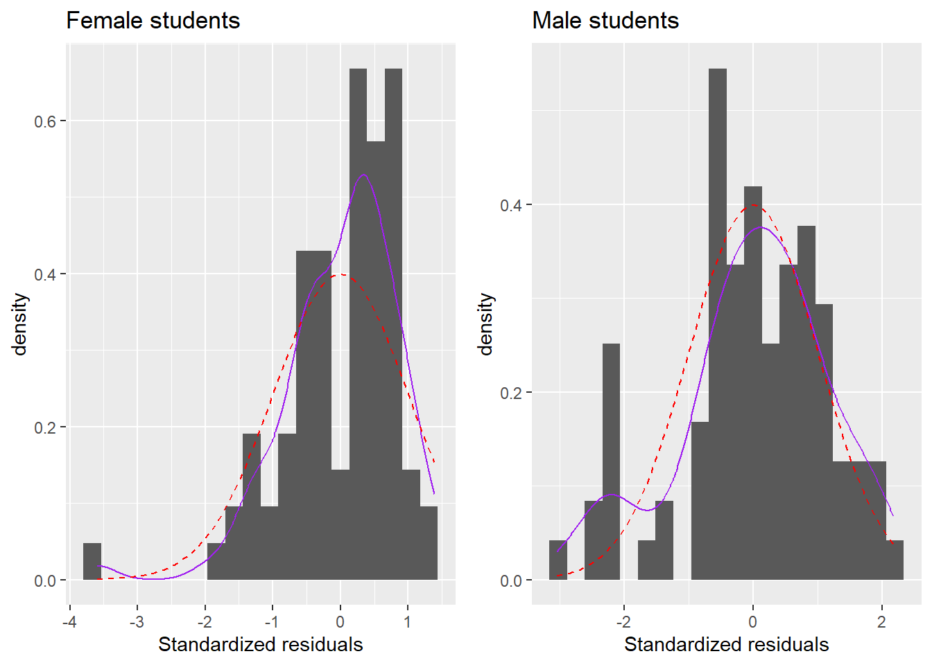
Figure 3: Model assumption checking.
In Figure 3, there’s evidence against the assumption of normality. Boys and especially girls have residuals which are too negative to be reasonable if the assumption of normality were met. Also, girls don’t have enough large positive residuals, possibly because of some sort of ceiling effect.
We can check the assumption of homoscedasticity by calculating the variance of the residuals for girls (\hat{\sigma}^2_{\varepsilon,girls}=0.70) and boys (\hat{\sigma}^2_{\varepsilon,boys}=1.30). Once again, there’s evidence that the assumptions are not met, because the residuals for boys appear to be more variable than the residuals for girls. We can test this using a Levene’s test of equality of variance, which tests a null-hypothesis that the variances of the outcome are the same in the two groups in the population; we reject the null hypothesis (F_{1,169}=6.58, p=.011) and conclude that the residuals are more variable for boys than for girls (we’re not using this test in this class, this is just an illustration).
However, when we rerun our analyses using either robust standard errors or a bootstrap, we obtain similar results, so these model assumption violations were probably not a problem for our analysis.
When we have additional predictors, we can no longer take it for granted that the assumption of linearity is met. We check the assumptions in the same way we discussed in chapter 8. If we want to be especially careful, we can conduct the tests first looking at the residuals for only female respondents, and then looking at the residuals for only male respondents.
Displaying our results
We need a way to display our results. As always, we want a plot which is visually compelling and easy to understand, and which addresses our research question. With a dichotomous predictor and a substantively interesting numeric predictor, one good choice is to plot the outcome against the numeric predictor, plotting two lines, one for each group of the dichotomous predictor.
Code
dat$labels <-factor(dat$male, levels =0:1, labels =c('F', 'M'))cols <-c('blue','pink2')mod <-lm(emp_scale ~ safe_scale + male, dat)coefs <-coef(mod)ggplot(dat, aes(x = safe_scale, y = emp_scale)) +geom_text(aes(label = labels), col = cols[dat$male +1]) +geom_abline(intercept = coefs[1], slope = coefs[2], col = cols[1]) +geom_abline(intercept = coefs[1] + coefs[3], slope = coefs[2], col = cols[2]) +xlab('Sense of safety at school') +ylab('Empathic concern')
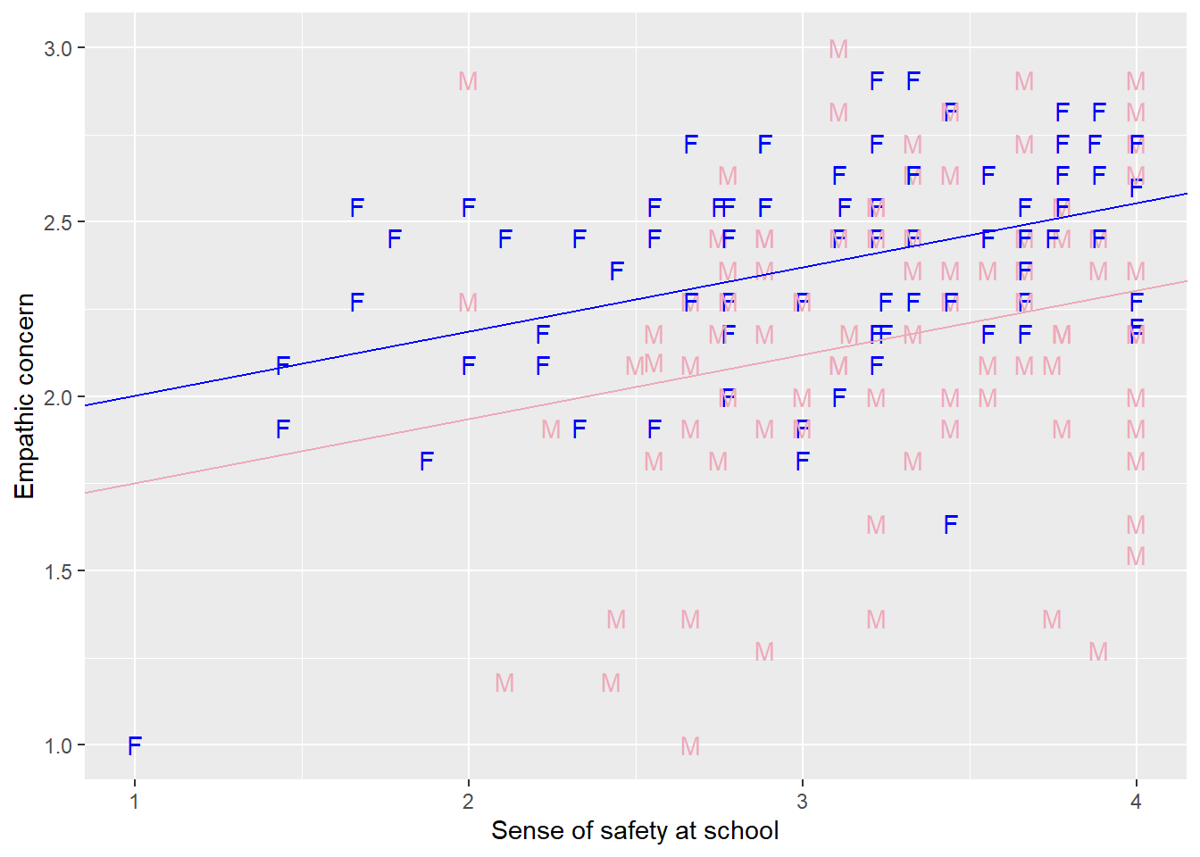
Figure 4: Estimated line of best fit of EMPATHY on SAFETY for boys (pink2) and girls (blue).
Figure 4 shows the plot. We’ve also added the scatterplot. Notice that our previous observation, that boys report a much wider range of empathic concern than girls, using the low end of the scale far more than girls, is reconfirmed.6
Summary
We wanted to address two research questions: first, do girls or boys report higher levels of empathic concern? Second, do girls or boys report higher levels of empathic concern when controlling for how safe they feel at school (or do students who feel safer at school report different levels of empathic concern, controlling for gender)?
Code
M1 <-lm(emp_scale ~ male, data = dat)M2 <-lm(emp_scale ~ safe_scale, data = dat)M3 <-lm(emp_scale ~ male + safe_scale, data = dat)htmlreg(list(M1, M2, M3), ci.force =TRUE, custom.coef.names =c('Intercept','MALE','SAFETY'))
Table 1: Statistical models predicting empathic concern. This table was automatically generated using the R package texreg.
Statistical models
Model 1
Model 2
Model 3
Intercept
2.38*
1.80*
1.82*
[ 2.29; 2.46]
[1.50; 2.10]
[ 1.53; 2.11]
MALE
-0.21*
-0.25*
[-0.33; -0.09]
[-0.37; -0.14]
SAFETY
0.15*
0.18*
[0.05; 0.24]
[ 0.09; 0.28]
R2
0.07
0.05
0.15
Adj. R2
0.07
0.05
0.14
Num. obs.
167
167
167
* Null hypothesis value outside the confidence interval.
Table 1 displays the results of several regressions that we fit. The negative coefficient for MALE in model 1 indicates that girls report higher levels of empathic concern, and this remains true when adjusting for sense of safety at school, as we see in model 3. In model 2, we note that students who feel safer in school report higher levels of empathic concern, and this remains true when adjusting for gender. However, none of the models explain more than 15% of the variation in empathic concern, indicating that the bulk of variability in empathic concern is not predicted by either gender or sense of safety.
Appendix
The problem with dichotomous outcomes
We’ve been focusing on using dichotomous variables as predictors, through the creation of indicator variables. However, we might also be interested in using dichotomous variables as outcomes, for example regressing an indicator for college graduation on predictors. It might seem straightforward to include an indicator variable as an outcome. Remember that regression tries to estimate \mu_{Y|X}, the mean of Y at some value of the predictors, X. The mean of an indicator variable is the proportion of people who have a 1 for the variable, or the probability that a person will have a 1, which is totally a sensible thing to predict in a regression.
But there are some problems. First, the distribution of the residuals cannot possibly have a normal distribution at each value of the predictor. Every residual will be either -\mu_{Y|X}, if the respondent has a 0, or 1-\mu_{Y|X}, if the respondent has a 1. Second, the residuals will not be homoscedastic. Recall that, for an indicator variable, the variance is equal to \mu_{Y|X}(1-\mu_{Y|X}). But this means that the variance of the residuals is a function of the mean, and so is not constant. Finally, the linear model probably isn’t right; in particular, probabilities have to be between 0 and 1, but there’s no way to force a linear regression model to constrain its predictions to be between those values; draw the line out far enough and it will go below 0 or above 1.
Despite these limitations, regressions predicting dichotomous outcomes, which are known as linear probability models, sometimes make sense, especially when coupled with robust standard errors. A better approach is known as logistic regression, which is a special case of a generalized linear model, but we don’t cover the topic in these notes.
Identifiability
One thing that’s confusing for many new analysts is why we only enter a single indicator variable for each grouping into a regression. Why not create a second indicator, FEMALE, and fit the model
The reason is something known as identifiability. We’ll illustrate. Recall from before that the mean value of empathic concern for girls is 2.38, while the mean for boys is 2.16. Obviously we want our model to have coefficients (\hat{\beta}_0, \hat{\beta}_1, and \hat{\beta}_2) such that \hat{\mu}_{girls}=2.38, and \hat{\mu}_{boys}=2.16. One way to get those predictions would be to let \beta_0=0, \beta_1=2.16, and \beta_2=2.38. Another way would be to let \beta_0=2.38, \beta_1=-0.22, and \beta_2=0 (this is the model we estimated above). Yet another would be to let \beta_0=2.16, \beta_1=0, and \beta_2=0.22. In fact, there are an infinite set of possible fits, all of which reproduce the sample means, and therefore minimize the variance of the residuals. We have no way of selecting among these models, and so we say that the model is not identified. This is sort of the mother of all collinearities, where two predictors are perfectly correlated, and it will seriously mess up your models. But most statistical software will handle the problem by dropping one of the problematic predictors and sending you a warning.
The assumption of linearity
One nice thing about a simple linear regression on an indicator variable is that the assumption of linearity is always met, because we can always connect a pair of means (i.e., the mean of the outcome for respondents for whom the indicator variable is zero and the mean for respondent for whom the indicator variable is 1) with a straight line.7 Given that the assumption of linearity is so important, it’s nice to know that we can always meet it, as long as we’re willing to dichotomize our predictors. For example, if we’re not sure that the association between age and reading comprehension is linear, we can dichotomize age (maybe by creating an indicator variable for being above the median age) and regressing reading comprehension on the indicator). On the other hand, this subtly changes the research question and throws away a great deal of information about the predictor. It also only works for simple linear regressions, as we’ll discuss in the section on interactions.
Effect sizes
When working with scales we don’t understand, interpreting the magnitude of regression coefficients can be challenging. For example, if we don’t know what 0.22 on the empathic concern scale means, how meaningful is it to say that girls have EMPATHY values 0.22 higher than boys?8 One thing we can do to make the coefficient more meaningful is to put the outcome on a standardized scale, by dividing it by its standard deviation (and possibly first subtracting the mean). Then the regression coefficient is the estimated mean difference between girls and boys in standard deviation units. Don’t standardize the indicator variable, MALE. We refer to this difference as an effect size. We know the meaning of a one-unit difference in the indicator (i.e., male students v.s. female students), and standard deviation units are almost never helpful for indicator variables.
When we regress the standardized empathy score on gender, we obtain the following fitted model:
EMPATHY^{std}_i = 0.28 - 0.55MALE_i,
indicating that boys report values of empathy 0.55 standard deviations lower than girls.
Be careful in interpreting these results. A large standardized difference means that a large portion of the variance in the outcome is attributable to group membership. However, it doesn’t tell us if the difference is substantively important.
Treatment effects
One situation which frequently calls for indicator variables is in estimating treatment effects. Suppose that we have a dataset consisting of people who were assigned to treatment and people who were assigned to control. Suppose we have a variable, T, which is equal to “treated” or “control” depending on each person’s treatment assignment. Then let Z_i be an indicator variable for assignment to the treatment condition such that
We refer to Z_i as a treatment indicator, since it’s an indicator for being assigned to treatment. Notice that the control group is in the reference category.9 Now we can fit the model
Y_i = \beta_0 + \beta_1Z_i + \varepsilon_i.
In this model \beta_0 represents the mean value of controls on the outcome, and \beta_1 represents the mean difference between treated and control units, which is also known as the treatment effect.
This is the exact same as a t-test. But we can improve our precision by adding controls. Remember if we add controls which
explain variance in the outcome and
are not correlated with the predictor of interest (Z_i)
then we should be able to estimate \beta_Z (often written as \tau) more precisely, which is a good thing. So we might get better results if we can add predictors which are strongly associated with the outcome. Adding controls doesn’t change our interpretation of the treatment effect because they should be perfectly uncorrelated with treatment assignment. This only works when the sample is sufficiently large; in small samples including controls can introduce bias into our estimates of the treatment effects, even when treatment is actually assigned at random.
Footnotes
Our conception of gender is rapidly expanding to include other categories, and we could plausibly conceive of a femininity or masculinity scale. On the other hand, given how attached society is to the binary construction of gender, it might be more appropriate to continue to treat gender as a dichotomy for reserch purposes.↩︎
Some people call these ``dummy’’ variables, but we know that only a real dummy calls other variables dummies. So there.↩︎
This is another way of stating that the linear model is correct, which is always the case in a simple linear regression with a dichotomous predictor. The appendix goes into this in more detail.↩︎
As we mentioned before, this is because we assume that all students are girls or boys. If there are students to whom these labels do not apply, units with a 0 on the MALE variable would be anyone who is not male. This is an important point: the reference category in a regression is anyone who has a 0 on the indicator variable; depending on how the indicator variable is defined this may be a meaningful group, or it may not.↩︎
You might wonder why we forced you to learn how to do t-tests given that you can do the same thing with regression; we prefer to think of it as giving you the purely gratuitous opportunity to learn how to do t-tests. You lucky ducks!↩︎
Though one girl reported an extremely low value of both empathy and safety.↩︎
This actually requires the very technical and reasonable assumption that the mean of the outcome conditional on the values of the indicator variable actually exists. Also, a steady hand or a straightedge to help you connect the dots.↩︎