These course notes should be used to supplement what you learn in class. They are not intended to replace course lectures and discussions. You are only responsible for material covered in class; you are not responsible for any material covered in the course notes but not in class.
Overview
The setting
Polychotomies
Regressing on polychotomies
Polychotomies and inference
Correcting for multiple comparisons
Adding controls
Appendix
The setting
We’ll continue working in the same setting. However, this time, we’d like to know if empathic concern is associated with students’ self-reported values. In another part of the survey, students were asked to rank three values, achievement, personal happiness, and caring for other people. We’ve created a variable VALUE, which identifies which of these values was most important to the student. We’d like to see if this is related to empathic concern, specifically whether students who report that caring for others is most important to them also report the highest levels of empathic concern; we don’t have any hypotheses about how students who rank personal happiness or achievement first will differ in empathic concern, only that they should be lower than students who ranking caring for others first.
Code
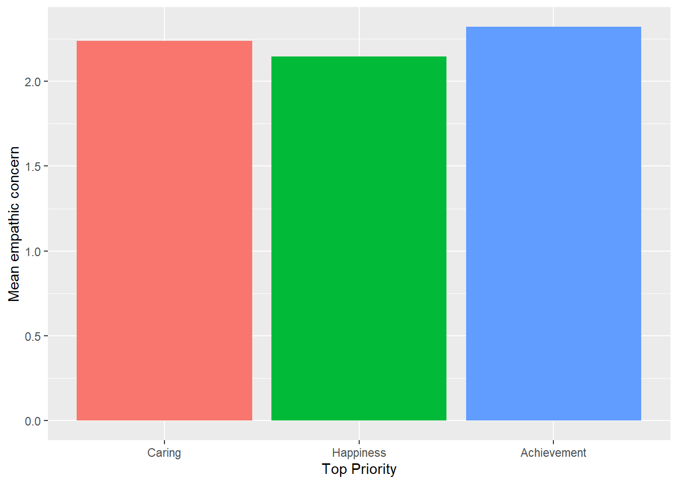
bar_dat <- dat %>%group_by(qual_most) %>%summarize(val =mean(emp_scale, na.rm =TRUE))ggplot(bar_dat, aes(x = qual_most, y = val, fill = qual_most)) +geom_col() +guides(fill ='none') +ylab('Mean empathic concern') +xlab('Top Priority')
Figure 1: Mean empathic concern by student priority.
In this school, 38 students selected “caring” as their most important value, while 29 students selected “happiness” and 105 selected “achievement”. Students who prioritized caring had a mean value of EMPATHY of 2.24, while students prioritizing personal happiness had a mean of 2.15, and students prioritizing achievement had a mean of 2.32.
Figure 1 displays mean reported empathic concern by students’ self-identified priorities. A quick glance should make it clear that our hypothesis will not be confirmed. Still, it’s worth investigating a little further.
Polychotomies
As you’ve probably noticed already, we’re running into a similar problem as in the previous unit. We can’t regress empathic concern directly on VALUE, because the individual values are things like “achievement”, and “caring”, and \beta_1 \times achievement isn’t a meaningful expression. On the other hand, VALUE isn’t dichotomous, so we won’t be able to use quite the same trick of creating an indicator variable to represent VALUE (though we’re going to do something very similar). A single dichotomy can’t possibly represent a variable which assumes three different values.
If the only thing we want to do is compare students who think caring for others is most important to all other students, we might change VALUE slightly to have only two levels: “caring” and “something else”. Then we could proceed by creating an indicator variable, CARE, which would have a value of 1 for anyone who put caring as the top value, and 0 for everyone else. We could then proceed exactly as we did with gender.
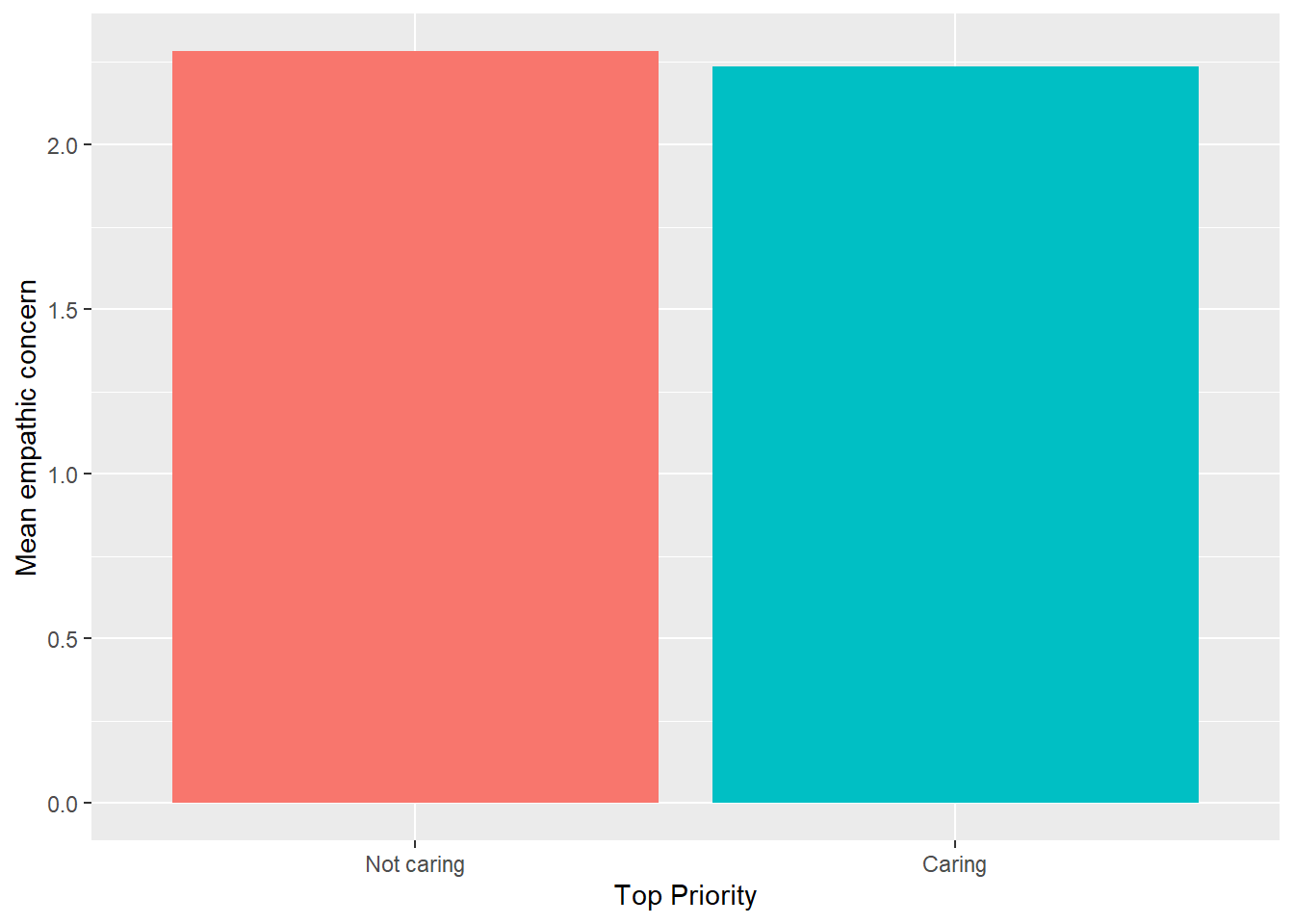
Notice that the reference category is respondents who do not rank caring for others first. The fitted model is
\hat{EMPATHY}_i = 2.28 - 0.05CARE_i.
Just to practice, we can interpret this as saying that respondents who do not rank caring first (the reference category) express a mean empathic concern of 2.28 scale points. Respondents who do rank caring first, express a mean empathic concern 0.05 scale points lower than those who do not. Figure 2 represents this model; one bar shows the mean empathic concern for respondents who put caring first and the other shows the mean for everyone else.
Figure 2: Mean empathic concern by student priority.
There are three problems with this approach. First, although our research question is primarily about comparing people who prioritize caring to all others, it would also be interesting to see if people who prioritize achievement differ from those who prioritize personal happiness. Second, if we found a difference in mean empathy between those who prioritize caring and those who don’t, we wouldn’t know if people who prioritized personal happiness and people who prioritized achievement both differed from those who prioritized caring, or if it was only one group. Finally, we don’t expect the mean value of empathic concern to be the same for people who prioritize achievement and people who prioritize personal happiness. Lumping these two groups into a single category, “something other than caring first”, could lead to largish residuals in that group, which will inflate \hat{\sigma_\varepsilon}, and lead to less precise inferences; our predictions won’t be as accurate as they could be, and so our inferences won’t be as precise as they could be.
So what we’d like is an analytic approach which allows us to treat the three different levels of the VALUE variable as three distinct groups. Ideally, this will build on the approach we developed for dichotomies, because we understand that fairly well and we’re just too lazy to learn something completely new.
Here’s the approach we’re going to take: we’re going to create a set of three indicator variables, which we’ll call CARE, ACHIEVEMENT and HAPPINESS. These variables assume a value of one for students who selected that value as the most important, and zero for students who selected something else. For example, suppose that student i selected caring as her most important value. Then CARE_i=1, ACHIEVEMENT_i=0, and HAPPINESS_i=0. Note that every student who responded to the item will have a one for exactly one indicator variable, and a zero for the other two. There’s no way to have a 0 for every indicator; that would mean the student didn’t select any value and we would treat that response as missing. There’s also no way to have a 1 for more than one indicator; that would mean the student ranked more than one value as most important which they were not permitted to do on the survey.1
The set of these three indicators, CARE, ACHIEVEMENT, and HAPPINESS, collectively capture all of the information in VALUE. In fact, any two of those indicators give us enough information to completely reconstruct VALUE. If we take, say, ACHIEVEMENT and HAPPINESS and observe that a respondent has a 1 on ACHIEVEMENT, we know that she or he ranked achievement first. If she has a 1 on HAPPINESS, she ranked personal happiness first. If she has a 0 for both ACHIEVEMENTandHAPPINESS, she must have put caring about others first.
Regressing on polychotomies
Now we need to use the indicator variables to represent a polychotomy in a regression model. As we noted before, we can’t use the model
This allows us to represent a polychotomy with two indicator variables.
We’ll briefly discuss how to interpret the coefficients, and then discuss some other ways we could parameterize this model.
First we’ll consider the intercept. The intercept, \beta_0, is the mean value of EMPATHY for respondents who has a zero for both HAPPINESS and ACHIEVEMENT. But thinking back to how we defined the indicator variables, these are the respondents who selected ``caring’’ as the most important value; remember, if a respondent has a 0 for both ACHIEVEMENT and HAPPINESS, it’s because she put CARING first.
Now consider respondents who identified ``happiness’’ as their most important value. These respondents will have zero for ACHIEVEMENT, and one for HAPPINESS. The equation for them will be
This is equal to the mean value for respondents who prioritized caring (\beta_0), plus \beta_1. So \beta_1 is the mean difference in empathic concern between respondents who prioritized happiness and respondents who prioritized caring. Notice how similar this is to how we’ve interpreted other coefficients of indicator variables.
Following a parallel argument, \beta_2 is the mean difference in empathic concern between respondents who prioritized achievement and respondents who prioritized caring. Notice that none of the coefficients directly measures the mean difference in empathic concern between respondents who prioritize happiness and respondents who prioritize achievement. However, we could obtain this difference by taking \beta_1-\beta_2. Alternately, we could fit either
(in which people who prioritize happiness are in the reference category) in which case \beta_1 or \beta_2, respectively, would be the difference we were interested in.
As with a dichotomous predictor, we refer to the group which doesn’t contribute an indicator variable to the model as the reference category or reference group, because all of the coefficients in the model, except \beta_0 refer to differences in the outcome between one group and the reference group. Also as with a dichotomous predictor, we have to leave out one indicator variable in order for the model to be identified (see the appendix). One way to understand this is to remember that we capture all of the information in VALUE using only two of the indicators. Adding the third adds no new information whatsoever, which means that it can’t contribute anything to the model.
Because we’re primarily interested in comparing students who prioritize caring to all other students, our preferred model is
If we wanted to compare students who prioritized achievement to all other students, we would make them the reference category. However, a model which omitted ACHIEVEMENT in favor of CARE would give the exact same fit in terms of R^2 and \hat{\sigma}_\varepsilon, and it would be possible to calculate all of the coefficients of one model using only the coefficients of the other.
In the current example, the fitted regression model is
We could have predicted this already, given the mean values of EMPATHY for students who prioritized caring, personal happiness, and achievement, which we presented above. The mean for students who prioritized caring was 2.24 (i.e., \hat{\beta}_0). The mean for students who prioritized personal happiness was 2.15 (i.e., \hat{\beta}_0+\hat{\beta}_1). Finally, the mean for students who prioritized achievement was 2.32 (i.e., \hat{\beta}_0+\hat{\beta}_2).
Polychotomies and inference
In this analysis, the p-value associated with \beta_1 (happiness) is .356; the p-value associated with \beta_2 (achievement) is .273.3 So there’s really not much evidence at all that students who prioritize caring report different levels of empathic concern than students who prioritize either personal happiness or achievement. Since our original research question was whether students who prioritized caring differed on average in empathic concern from either of the other two groups, it looks like our answer is going to be that there’s no evidence of a difference.
But notice that students prioritizing achievement report higher levels of empathic concern than students prioritizing caring, and students prioritizing personal happiness report lower levels. So maybe we have evidence that those two sets of students, students prioritizing personal happiness and students prioritizing achievement, actually do differ in the population on mean empathic concern.
Our current model doesn’t make this easy to test.4 However, we’ve already proposed two alternative models above which contain coefficients which directly represent the difference in mean empathic concern between students prioritizing achievement and students prioritizing personal happiness. For example, in the model
we’ve taken students who prioritize achievement as the reference category, and now \beta_1 represents the difference in mean empathic concern between these students and students who prioritize personal happiness.
When we fit this model, we obtain
EMPATHY_i = 2.32 - 0.17HAPPINESS_i - 0.08CARE_i.
Once again, we should have been able to calculate the coefficients directly from the mean reported values of empathic concern, or from the first model, but the p-values are harder to get.
In this new model, the p-value for \beta_2 is, of course, .273.5 However, the coefficient of \beta_1 is .038, which is below our \alpha threshold of .05. So we have sufficiently convincing evidence that, on average in the population, students who prioritize achievement report higher levels of empathic concern than students who prioritize personal happiness.
This may seem strange at first, and can help to foreground a common mistake in statistical inference. A naive data-analyst might identify this as paradoxical using the following line of reasoning.
In our first model we found that neither students prioritizing personal happiness nor students prioritizing achievement differed, on average in the population, from students prioritizing caring.
Therefore students prioritizing personal happiness and students prioritizing achievement report the same mean levels of empathic concern in the population.
But our third model showed that this is not true, and that students prioritizing achievement actually report higher levels of empathic concern than students prioritizing personal happiness, which directly contradicts the previous result.
Can you spot the errors? The first, and probably most problematic, is in the first line. We didn’t find that “neither students prioritizing personal happiness nor students prioritizing achievement differed, on average in the population, from students prioritizing caring”, we simply found no convincing evidence that they did differ. These are very different things! We certainly can’t conclude that “students prioritizing personal happiness and students prioritizing achievement report the same mean levels of empathic concern in the population”. And it’s also not true that “students prioritizing achievement … report higher levels of empathic concern than students prioritizing personal happiness”. We’ve found evidence of a difference which is fairly convincing, given the threshold we adopted (\alpha = .05). However, it’s entirely possible that this is a chance result and that, in the population as a whole, students prioritizing personal happiness don’t differ from students prioritizing achievement in empathic concern.6 Remember: the failure to find an association does not imply that there is no association, and the fact that we found evidence of an association does not guarantee that it exists in the population.
Correcting for multiple comparisons
There’s a reason that we might be reluctant to put too much faith in the difference we found between students prioritizing achievement and personal happiness. Remember: if a null-hypothesis is true, we should have a 5% chance of rejecting it and “finding” an association just due to chance, as long as we set \alpha = .05. What that means is that if we test a lot of null-hypotheses, all of which are true, we have a inflated chance of rejecting at least one of them by chance alone. If we test 20 true null-hypotheses, we should expect to reject an average of one of them just by chance.
In this example, we’ve essentially tested three null-hypotheses: first, H_0:\mu_{care}=\mu_{achieve}, second H_0:\mu_{care}=\mu_{happy}, and third, H_0:\mu_{achieve}=\mu_{happy}. So if all of these null-hypotheses are true, the probability that we will reject at least one of these null-hypotheses is greater than .05.
To illustrate this idea, we conducted a simulation. We began by creating an artificial population where all of the null hypotheses were true, and \mu_{care}=\mu_{achieve}=\mu_{happy} (that is, students have the same mean value of empathic concern, no matter which value they prioritize). We then took 10,000 samples of students, with each sample containing 105 students prioritizing achievement, 38 prioritizing caring, and 29 prioritizing personal happiness. In each sample, we recorded the number of significance tests which (incorrectly) rejected H_0. Across all samples, we rejected, as expected, close to 5% of the null hypotheses (4.8%, to be precise). However, in 8.75% of the samples we rejected at least one null hypothesis.
If our goal is not to control the Type-I error rate for a particular test, but to control the error rate for a group of tests, then we need to alter our p-values to correct for the fact that multiple tests increase the number of Type-I errors we commit. A common correction is known as the Bonferroni correction. It’s popular because it’s simple and because it doesn’t make any assumptions about how the different tests are related to each other. We conduct a Bonferroni correction by multiplying each p-value by the number of tests we’ve conducted, or, equivalently, divide \alpha by the number of tests. This will reduce the Type-I error rate both for each test, and for the group of tests as a whole.
In our example, we conducted three tests, so we would multiply the p-values by three or divide \alpha by three. Either way, we need a raw p-value of .05/3=.017 before rejecting a given null-hypothesis. In our simulation, we reject 1.6% of our null-hypotheses, as we expect. We reject at least one null-hypothesis in 3% of our simulations, which suggests that we may have actually overcorrected (the Bonferroni correction tends to be overly conservative, meaning that it rejects true null-hypotheses even less often than it aims to).
Deciding when to apply a correction is more of an art than a science, and the decision often depends on the traditions of your field. If we keep in mind that we will falsely reject 5% of true null-hypotheses, it’s not always clear what we gain from correcting at all. On the other hand, if our main finding is that there’s at least one difference (e.g., that a treatment affected at least one outcome), then it probably makes sense to correct our p-values.
Adding controls
As in previous chapters, it frequently makes sense to add control variables to our models. In this example, we’re going to estimate the association between empathy and values, controlling for respondent gender. The model we’ll fit looks like this (we’re going to switch to students who prioritize achievement as the reference category for the purpose of illustration):
We’ve made this point before, but want to stress is again because it’s so important. The coefficients \beta_0, \beta_1, and \beta_2 no longer represent the same things as in the previous model. Before, \beta_1 represented the average difference in empathy between all students who prioritized happiness and all students who prioritized achievement. Now it represents the average difference in empathy between girls (or boys) who prioritized happiness and girls (or boys) who prioritized achievement. If girls and boys prioritize happiness and achievement at different rates, \beta_1 might be very different in this new model because it represents something very different. This doesn’t only mean that our estimate, \hat{beta}_1 will be different, but also that the thing which is being estimated, \beta_1, will be different.7
The coefficients for HAPPINESS and CARE haven’t changed much, but boys with the same priorities as girls report lower levels of empathy. The coefficient of CARE is still not significant, but the p-value for the coefficient of HAPPINESS is now .017. After applying a Bonferroni correction and multiplying the p-value by 3, the corrected p-value is 0.051, which is very close to the conventional level of statistical significance. The reason the p-value got smaller is that including gender as a predictor slightly increased the estimated coefficient and slightly decreased the associated standard error because gender explained some of the residual variance. If we feel a need to correct for multiple tests, we have a great deal of evidence against a null-hypothesis H_0:\beta_1=0, though not quite enough to reject it based on conventional standards.
Appendix
Polychotomies and ANOVAS
You may be familiar with the term Analysis of Variance, or ANOVA. Although the term covers a wide range of possible analyses, the traditional ANOVA entails trying to see whether variance in an outcome can be associated with levels of a categorical predictor (or set of categorical predictors). That should sound familiar to you, since that’s exactly what linear regression on a polychotomous predictor does. Some of the terminology is different, and ANOVA models are specified slightly differently than how we usually fit regression models, but the underlying mechanics are identical.
We prefer to work within a regression framework as opposed to an ANOVA framework for several reasons. First, we find that regression models extend more readily to control for numeric predictors; this can be done using ANOVA, but it’s less straightforward. Since we usually obtain better predictions and clearer results using numeric predictors, this is a plus. Second, we like the emphasis that regression put on prediction of outcomes and association between outcomes and predictors. Although ANOVA is doing the same thing as regression, we find that the language used in ANOVA sometimes distracts us from the real goal of the analysis; in ANOVA, estimating the controlled associations between predictors and outcomes often seems secondary to estimating whether there’s any association at all. Third, regression is the approach of choice in a number of disciplines closely related to education, including economics and sociology.
On the other hand, there are advantages to being familiar with ANOVA as well. It’s used extensively in psychology, which is another cornerstone of education. We also enjoy the clean way in which ANOVA represents categorical variables. A model which usually looks like this in regression:
Regardless, it’s handy to know both frameworks, if only to make it easier to read journal articles in different fields.
Selecting the reference group
One choice you have to make when working with categorical variables, and to a lesser extent dichotomous variables, is which category to treat as the reference. Sometimes this is a straightforward decision, driven by the research agenda. In this unit, we were interested in comparing students who prioritized caring to students with different priorities. The only model which allows us to make these comparisons directly is one where students who prioritize caring are the reference group. In other cases, such as when the categorical predictor is only being used as a control, the decision won’t be as obvious.
It can be useful to treat the largest group as the reference, because that will tend to give you more power in your analyses because the standard error for the mean score for the reference group will tend to be small. Another option is to simply take the first group (in alphabetical order) as the reference.
One unfortunate approach adopted by some researchers is to automatically select the socially favored group as the reference. For example, researchers frequently treat white, heterosexual males as the reference category. This has the unfortunate effect of suggesting that this is the group against which all others must be measured. Certainly there will be cases where the research question requires that white, heterosexual men be the reference category. However, if you find that this is always your reference group, you might rethink your approach to generating research questions.
Regardless, remember that reparameterizing your model by selecting different reference groups can give you a more complete picture of the associations in your data.
Other corrections
The Bonferroni correction is popular because it’s simple to apply, and guarantees an overall Type-I error rate of \alpha or less. However, as we saw in the simulation, it can be too conservative, and sometimes far too conservative. Here we discuss two other options.
The first is a bootstrap, but a very different bootstrap than the ones we’ve seen so far. In this bootstrap approach, we begin by creating a null-population as close to the sample as possible (in our current case, we would add or subtract a constant to each value in students outside of the CARING group so that all of the means were identical). We then take repeated bootstrap samples with replacement, and fit the model in each sample. From each fit, we store the lowest p-value (remember, these are p-values from a population where the null-hypothesis is true). We then reject any null-hypothesis in the original sample where the p-value is less than all but \alpha (5%) of the bootstrap p-values. The logic is that any p-value we reject is one that is more extreme than all but 5% of the smallest p-values we would have gotten sampling from a null-population. This will usually control the group Type-I error rate at the nominal level, and tends to be more powerful than the Bonferroni correction.
The second approach is to minimize something called the false discovery rate. The Bonferroni correction attempts to guarantee a group Type-I error rate of less than \alpha. In other words, it tries to guarantee that the probability of falsely declaring even a single association to be non-zero is less than \alpha, if all of the true associations are 0. This makes it extremely hard to find any associations whatsoever especially if we’re conducting a lot of tests. When using the false discovery rate as our criterion, we try to guarantee that the proportion of null-hypotheses that we reject which are actually true is less than \alpha. This means that if we’re finding a lot of true associations, we don’t mind mistakenly ``finding’’ some false ones. One way to control the false discovery rate is to use a Benjamini-Hochberg correction. This approach works as follows: begin by lining up the p-values to be corrected from smallest to largest. Suppose we have m p-values. If the first p-value is smaller than \frac{1}{m}\alpha, reject it. If the second is smaller than \frac{2}{m}\alpha, reject it. If the third is smaller than \frac{3}{m}\alpha, reject it. Continue through the list of p-values. Find the last p-value which was lower than the number we were comparing it to (we compare the kth pvalue to \frac{k}{m}\alpha). Reject every null-hypothesis associated with a p-value smaller than the kth p-value. This correction will reject more frequently than Bonferroni, because it is trying to control a different rate.
Fixed effects
Another common use for categorical predictors is fixed effects regression. Remember that one assumption we make is that residuals are independent of each other, and that this assumption may be violated when students are sampled from higher-order units. For example, if students are sampled from schools, students within the same schools may have similar residuals. One way to handle this assumption violation is to control for the school by adding a set of indicator variables which identify whether the student is enrolled in a particular school (as before, we leave out one school indicator for the sake of identifiability). This essentially removes any school-level differences from the outcome, making the assumption of independence much more plausible. We don’t cover fixed effects regression in detail in this course, but it’s a common approach, especially in economics.
Plots
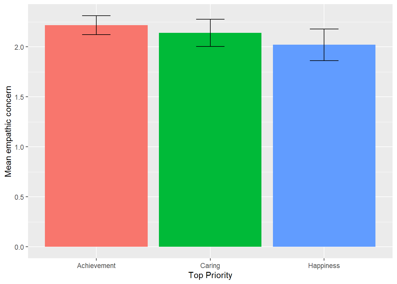
A useful plot when dealing with categorical predictors is a barplot with lines indicating \pm2 standard errors, to give your audience a sense of mean differences and the precision with which those differences have been estimated. @fig:emp_plot shows what that plot would look like for our final model.
Code
coefs <-coef(summary(lm(emp_scale ~-1+relevel(qual_most, ref ='Achievement') + female, data = dat)))tab <- coefs[1:3, 1]bars <- coefs[1:3, 2] *2bar_dat <-data.frame(Quality =c('Achievement', 'Caring', 'Happiness'), val =as.numeric(tab), bar =as.numeric(bars))ggplot(bar_dat, aes(x = Quality, fill = Quality, y = val)) +geom_col() +geom_errorbar(aes(ymin = val - bars, ymax = val + bars, width = .25)) +guides(fill =FALSE) +ylab('Mean empathic concern') +xlab('Top Priority')
Figure 3: Mean empathic concern by student priority controlling for gender with bars extending \pm2 standard errors.
You’ll notice that there’s considerable overlap between any pair of standard error bars. On the face of it, that suggests that it’s plausible that the population mean of empathy for people who prioritize happiness is the same as the population mean empathy for people who prioritize achievement. That’s strange because the coefficient associated with that difference was statistically significant. In fact, that’s a misinterpretation of the meaning of the errors bars. It’s true that it’s plausible that the population mean empathy for respondents prioritizing happiness is quite a bit higher than the estimated value. It’s also plausible that the population mean empathy for respondents prioritizing achievement is quite a bit lower than the estimated value. However, it’s highly implausible that both of those are true and that the population means for the two groups of respondents are the same.
This highlights another key point about working with statistics: uncertainties frequently fail to combine in straightforward ways. If you want to know the uncertainty associated with a particular parameter, you’re usually best off fitting a model which gives you the value directly, rather than trying to figure it out from another model, even if the two models are equivalent.
Footnotes
This means that some variables we may think of as polychotomies are not. Suppose we gave a survey on which we asked students to indicate their race by selecting as many racial categories as applied to them. A student might identify as both Black and American Indian, or as both White and Asian. Some students might not select any categories. In this case the different races are neither exhaustive nor mutually exclusive, and so they can’t create a polychotomy. We can try to dodge this issue by creating racial categories of multi-racial'' andnone’’, but the multi-racial category will end up lumping together people with very different racial backgrounds, and the other categories will exclude a lot of people who seem like they ought to fall into them (people who are both Black and American Indian will be excluded from either group). The appendix will talk about how we can handle this.↩︎
That’s a math joke! Ha ha! Obviously you can’t multiply something by a word!↩︎
You might have noticed that the p-value for the larger coefficient, \beta_1, is less extreme than the p-value for the smaller coefficient. This is because far more students prioritize achievement than personal happiness in this school. This allows us to estimate the population mean empathic concern for students prioritizing achievement more precisely, and gives more evidence of a population-level difference, even though the estimated difference is smaller.↩︎
Actually, it’s entirely possible to test the null hypothesis that students prioritizing achievement and students prioritizing personal happiness differ in mean reported empathic concern using the model we fit. S-052 will introduce the concept of a general linear hypothesis, which we can use for comparing null-hypotheses about combinations of coefficients; here we would testing a null-hypothesis that \beta_1 = \beta_2, or that \beta_1 - \beta_2 = 0. However, the automatic output that most programs will give you doesn’t make this a straightforward task. It’s much simpler to just refit the model so that one of the coefficients directly represents the difference.↩︎
“Of course” because this represents evidence against a null-hypothesis that students who prioritized achievement and caring have the same level of empathic concern, just like \beta_2 from the first model; they’re testing the same null-hypothesis, using the same data.↩︎
As in an earlier unit, it’s a little weird to talk about the population as a whole here. We’ve sampled the entire school, so we have access to the entire population of students in this school. We’ve also only sampled from this one school, so we can’t really talk about associations in the population of all US students. As we often do when we apply statistics to educational contexts, we’re going to wave aside this issue and pretend that there exists some population from which we’ve actually taken a random sample. Other authors have more sophisticated and technically demanding ways of viewing this issue, which we discussed briefly in Unit 1 (i.e. thinking of inference as testing a probability model rather than estimating to a larger population).↩︎
In statistics, the thing which we are estimating is called the estimand, the thing we use to estimate is is called the estimator, and the actual value we calculate is the estimate.↩︎