These course notes should be used to supplement what you learn in class. They are not intended to replace course lectures and discussions. You are only responsible for material covered in class; you are not responsible for any material covered in the course notes but not in class.
Overview
The setting
Quadratic associations
Dichotomous by continuous interactions
Continuous by continuous interactions
Appendix
Note that, although this chapter covers both quadratic associations and interactions, these topics are not closely related to each other. Quadratic associations are a way to capture one type of non-linear association, while interactions are used to allow one association to differ based on values of another variable. Both of these concepts will be covered in more detail in the unit, but for right now just notice that they’re very different things.
The setting
We’re going to continue using data from Making Caring Common (MCC). This time we’ll be working with the full dataset of over 9,000 students sampled from 33 schools from around the United States (along with a few international schools). We’ll continue to ignore the nested nature of the data. This means that our results will be a little hard to trust and will not be ready for publication; if you want to learn how to handle nested data in a reasonable way, consider taking S-052. Also importantly, we’re going to pretend that we sampled these schools from some wider population. In fact, that’s not really accurate. Rather, these are actually all of the schools (in the known universe) that agreed to work with MCC on this research. It’s quite possible that the results we present here would also hold in other schools, but our statistics don’t allow us to demonstrate that. Setting all of these caveats aised, the outcome will still be students’ self-reported empathic concern. In this unit, we’re going to try to address the following research questions:
what is the association between students’ grade levels and empathic concern; and
does the association differ between girls and boys?
Some research exists which demonstrates that girls and boys follow different trajectories in their development of empathy and empathic concern. In particular, adolescence and puberty seem to have different effects on boys and girls. This unit attempts to contribute to that literature.1
But before we examine differences between girls and boys, we’re going to try to develop a better understanding of how empathic concern is associated with student grade.
Code
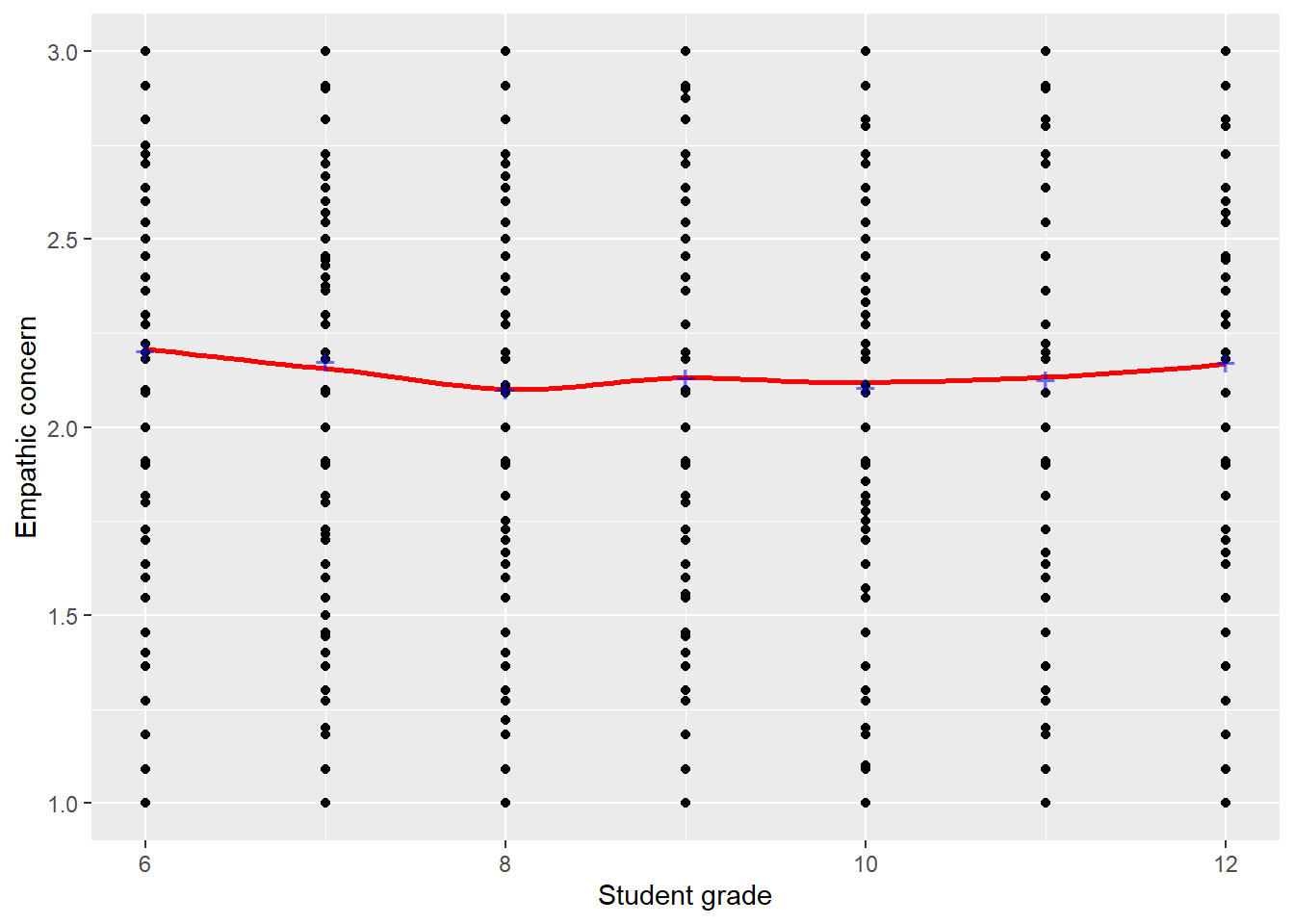
means <-data.frame(emp_scale =with(dat,tapply(emp_scale, grade, mean, na.rm =TRUE)))means$grade <-6:12ggplot(data = dat, mapping =aes(x = grade, y = emp_scale)) +geom_smooth(method ='loess', se =FALSE, col ='red') +geom_point() +geom_point(data = means, mapping =aes(x = grade, y = emp_scale, alpha = .5), col ='blue', cex =5, pch ='+') +xlab('Student grade') +ylab('Empathic concern') +theme(legend.position="none")
Figure 1: Mean empathic concern by student grade. LOWESS smoothed curve overlaid in red. Sample means for each grade represented as blue plusses.
Figure 1 displays the association between student grade and student empathic concern as measured by our scale. Notice that, although the association is very slight, there’s some evidence of a curvilinear relationship between the two variables. Students in the lowest and highest grades report the highest values of empathic concern; students in the middle grades (close to 9th grade) report the lowest.
We might be justified in treating this association as linear; the deviations from linearity are quite small, and a linear model is not wholly inappropriate. However, if we want to really capture the association between grade and empathic concern, we’d like to model the curvilinear relationship apparent in the data.
This is difficult to do. The association we see in the data is non-monotonic;2 from grade 6 to 9ish, the association is negative, and from grades 9ish to 12 it’s positive. Logarithmic transformations, the only kind we’ve covered so far, can make a steep association shallow or a shallow association steep. However they can’t transform a curve that rises and then falls into a straight line.
Quadratic associations
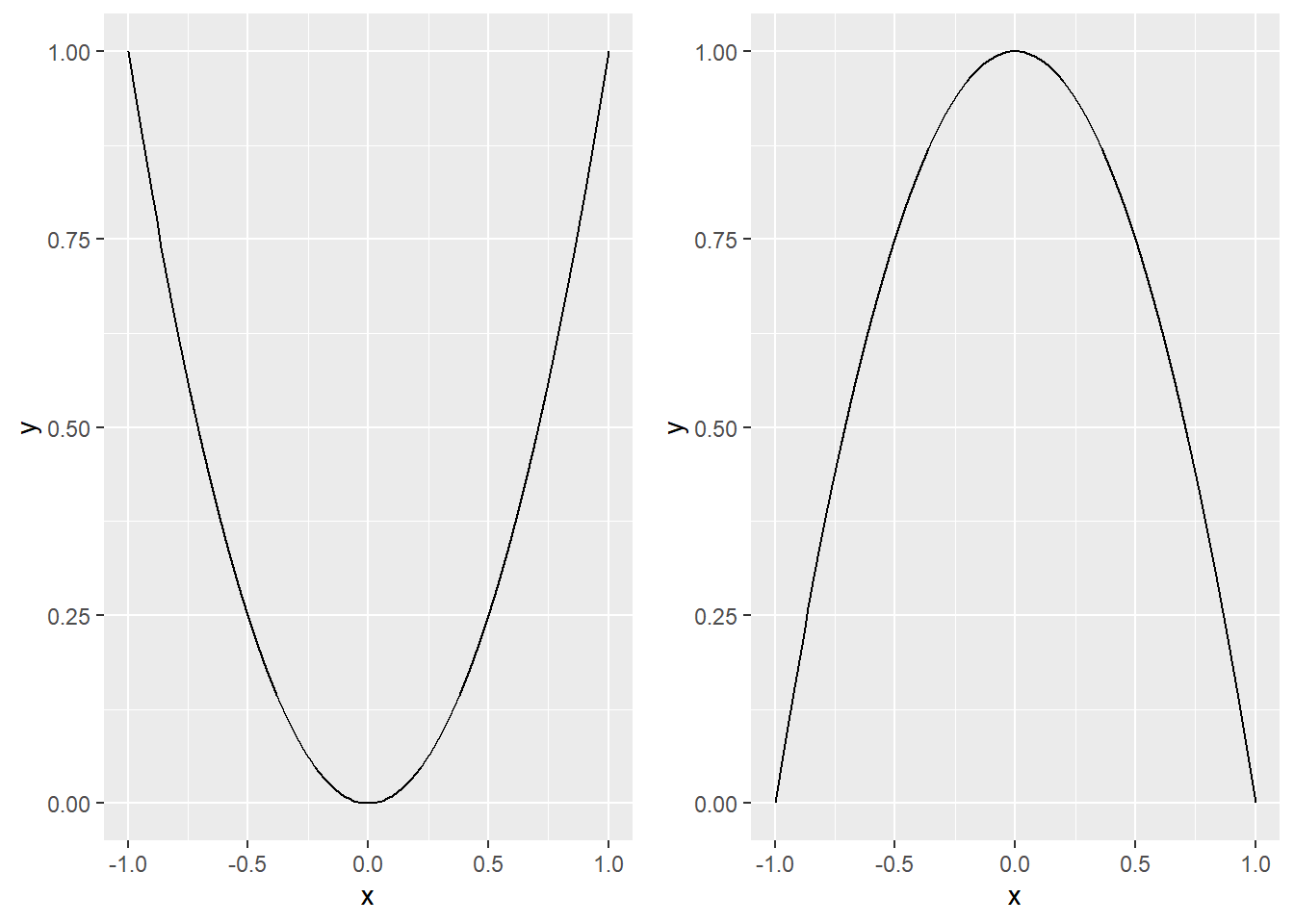
One association that does produce this sort of a curve is a quadratic association. Quadratic associations are curves with a single (or global) minimum or maximum value. As we move away from that value, the curve rises (or falls, depending on the exact quadratic curve we’re considering) more and more steeply. Figure 2 displays two possible quadratic curves, one of which opens downwards, the other of which opens upwards.
Figure 2: Two possible quadratic curves. The curve on the left opens downwards, while the one on the right opens upwards.
Quadratic associations are extremely useful for representing data where moderate values of the predictor are associated with the lowest (or highest) values of the outcome, and extreme values of the predictor are associated with the opposite. This is precisely what we see in Figure 1; students in the grades in the middle of the sample report the lowest values of empathic concern, while students in the lowest and highest grades report the highest values.
Every quadratic association can be described using the parameterization
y = ax^2 + bx + c
The leading coefficient, a, controls the general shape of the curve. Larger values of a give steeper curves, and negative values give curves that open downwards (curves with positive coefficients of x^2 open upwards). The coefficient of x, b, functions to shift the curve left or right; the minimum (or maximum) value of the quadratic is found at x = \frac{-b}{2a}. Finally, c shifts the entire curve up or down.
You may recall that we can also use the values of a, b, and c to calculate the values of x where the curve crosses the y-axis. However, this would be very unusual in statistics, in part because a value of 0 on the outcome is frequently not meaningful. In this application, for instance, it’s not possible to have a score lower than 1 on the empathic concern scale, so it’s not even possible for a student to have a 0.
To use a quadratic curve to model the association between empathic concern and grade, and taking EMPATHY as the outcome and GRADE as the predictor, we propose the following population model:
In this model, \beta_0 is equivalent to c, \beta_1 is equivalent to b, and \beta_2 is equivalent to a. EMPATHY is the outcome, y, and GRADE is the predictor, x. We obtain GRADE^2_i by squaring GRADE_i (so if a student is in tenth grade, she or he has GRADE = 10 and GRADE^2 = 100).
This is a population model which describes a quadratic association. Note that we can also use this model to represent a linear association: if \beta_2 = 0, then this model will describe a straight line.
When we fit this model to our data, we obtain the fitted model
All of the estimated coefficients are statistically significant with \alpha = .05. We are confident that these coefficients are not 0 in the population.
We interpret the intercept as before. It’s the estimated population mean value of empathy for students who are in grade 0.3 Of course, students with a value of 0 for GRADE must also have a value of 0 for GRADE^2, because 0^2 = 0.
Interpreting the slope coefficients is much more challenging. In most models we would interpret the coefficient of GRADE as the predicted difference in the outcome associated with a one grade difference, controlling for the other predictors. But since GRADE^2 is a function of GRADE, it’s not possible for two students to differ on GRADE but remain identical on GRADE^2. Similarly, if two students differ by one on GRADE^2, then they must differ on GRADE as well. What’s more, a one grade difference will be associated with a different difference in GRADE^2 depending on what GRADE is. Students in 6th and 7th grades differ by 1 for GRADE, and by 13 for GRADE^2 (7^2 - 6^2 = 49 - 36 = 13). In contrast, students in 11th and 12th grades also differ by 1 for GRADE, but differ by 23 for GRADE^2 (12^2 - 11^2 = 144 - 121 = 23). This is what gives a quadratic association its curvilinear nature, but it also complicates interpretation.
Here are two pieces of information we can extract from the fit. First, because \hat{\beta}_2 is positive, we know that the association has a global minimum value (rather than a global maximum). Another way to say this is that the curve opens upward. Second, if we take \frac{-\hat{\beta}_1}{2\times\hat{\beta}_2}, this gives us an estimate of the value of GRADE where the quadratic achieves its minimum value. In our case, this is equal to approximately 9.39, indicating that students seem to report the lowest value of empathic concern close to 9th grade.4 To be somewhat technical, this is a biased estimate of the population minimum, but should be reasonable in large samples.
For describing the association between GRADE and EMPATHY, we’re probably best off presenting a plot and describing the general shape. We can use the statistical significance of the quadratic term to test if there’s really a quadratic association between the variables; if not, we might prefer to just use a linear model.
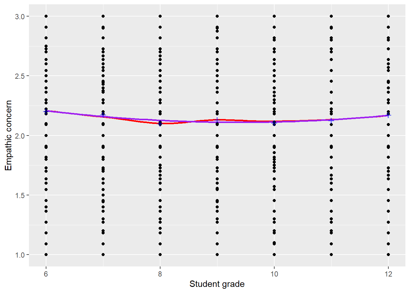
Figure 3 displays the model predicted association between EMPATHY and GRADE. It closely mirrors the LOWESS curve, though the LOWESS curve is consistently too high (this is somewhat technical, and doesn’t matter too much since we got the shape right). The curve is very shallow; mean empathy doesn’t have a strong association with grade and the model R^2 is only .005 (only half a percent of the variability in empathic concern is associated with grade). Still, we can clearly see the general curvilinear association, and the minimum near 9th grade.
Code
ggplot(data = dat, mapping =aes(x = grade, y = emp_scale)) +geom_smooth(method ='loess', se =FALSE, col ='red') +geom_smooth(method ='lm', se =FALSE, col ='purple', formula = y ~ x +I(x^2)) +geom_point() +geom_point(data = means, mapping =aes(x = grade, y = emp_scale, alpha = .5), col ='blue', cex =5, pch ='+') +xlab('Student grade') +ylab('Empathic concern') +theme(legend.position="none")
Figure 3: Mean empathic concern by student grade. LOWESS smoothed curve overlaid in red. Sample means for each grade represented as blue plusses. The purple line shows the association predicted by our model.
Dichotomous by continuous interactions
We can estimate the same association between EMPATHY and GRADE, but this time controlling for gender. Since girls and boys are more or less equally distributed across grade, we shouldn’t expect the estimated association between EMPATHY and GRADE to change, but we might get more precise estimates because including gender in the model will make our predictions better. The first model we might consider is
Note that this model treats girls as the reference category; \beta_3 estimates how boys differ from girls in the same grade (that is, adjusting for grade). The fitted model is
Notice that the estimated slope for GRADE and GRADE^2 are very similar to what we estimated in the original model. Again, we could have predicted this from the fact that gender is largely independent of grade level. The intercept has changed from 2.86 to 2.97; this is because the intercept is now estimating empathic concern for girls in grade 0, and on average girls report higher empathy than boys.5 The coefficient of MALE indicates that boys report empathy which is 0.21 scale points lower than girls in the same age, which is very close to the 0.22 scale point difference which we estimated in a previous unit. The p-value associated with GRADE is lower than it was before, because GENDER explains some of the residual variance, making our estimates more precise (remember, the more variable the residuals, the less precise our estimates).
One assumption that this model makes is that the coefficients for GRADE and GRADE^2 are the same for girls and boys. This is sometimes referred to as the main effects assumption, though we don’t like the use of the term “effect”, because it sounds very causal to us. This assumption may be correct, or may be approximately correct, or we may be willing to pretend that it’s correct (in which case we might think of \beta_1 and \beta_2 as averages across girls and boys). On the other hand, the regression framework allows us to explicitly test this hypothesis and to estimate a more flexible model where the association between empathic concern and grade differs for girls and boys. We’ll do this by adding something that we’ll refer to as an interaction.
In this model, the term MALE_i\times GRADE_i, which is formed by multiplying the two variables together, is called the interaction term. To see how this results in line fit independently for boys and girls, and to understand how to interpret the coefficients, consider what the equation would be for a female respondent. For this respondent MALE_i = 0, and
So \beta_4 and \beta_5 estimate the differences between the population coefficients for boys and girls. If these values are negative, then we estimate that the coefficients are lower for boys than for girls; if they are positive, we estimate that the coefficients are higher. We interpret p-values and standard errors just as before. Notice that \beta_3 represents the difference in the intercept between boys and girls. This is the estimated mean difference in empathic concern between boys and girls in grade 0, and remains meaningless. It may be tempting to think that \beta_3 is the estimated mean difference between boys and girls controlling for grade, but this is not correct; when two variables interact in a model, we need to change our interpretations of the coefficients of the variables.
The fact that \beta_4 was estimated to be 0.04 indicates that we estimate the linear coefficient of GRADE to be 0.04 more positive for boys than for girls (-0.14 v.s. -0.18). The fact that \beta_5 was estimated to be -0.003 indicates that we estimate the quadratic component of the model to be 0.003 more negative for boys than for girls (0.007 v.s. 0.010).6 In this example, neither \hat{\beta}_4 nor \hat{\beta}_5 was statistically significant at the .05 level, so we would probably omit them from our model.
In this model, the coefficients of GRADE, GRADE^2, and MALE are referred to as the main effects. This is a misnomer. The coefficients of GRADE and GRADE^2 are simply the coefficients for one subset of students, i.e., for girls. The coefficient for MALE is the coefficient for boys in grade 0 (otherwise the gender by grade interactions change the estimated difference between girls and boys). There’s nothing to make these estimates “main” in any reasonable sense of the word, except that the interactions are interpreted as deviations from these associations. Don’t be fooled into thinking that the main effects are somehow the real associations, or the most important associations. When two variables interact, the interpretation of the coefficients becomes quite complicated.
The interpretation of the interaction that we’ve given you, that the coefficients of GRADE and GRADE^2 differ by gender, strikes us as the most intuitive. However, it’s not the only possible way to view the model. We would be equally correct in saying that the association between gender and empathic concern differs according to grade; in some grades, girls and boys are more similar in reported empathic concern; in other grades they’re more dissimilar. This is mathematically equivalent to our first interpretation and equally valid, but we find it harder to explain, so we prefer to talk about the association between grade and empathic concern differing by gender. Ultimately, let the context govern your interpretation.
Table 1 displays all of the fitted models we’ve discussed. Note that we can handle interactions between dichotomous variables and other dichotomous variables, or between polychotomous variables and other variables using similar techniques, though interpretations can be much less clear.
Code
dat$EMPATHY <- dat$emp_scaledat$MALE <- dat$maledat$GRADE <- dat$gradedat$GRADE2 <- dat$GRADE^2dat$MALExGRADE <- dat$MALE * dat$GRADEdat$MALExGRADE2 <- dat$MALE * dat$GRADE2m1 <-lm(EMPATHY ~ MALE, data = dat)m2 <-lm(EMPATHY ~ GRADE + GRADE2, data = dat)m3 <-lm(EMPATHY ~ MALE + GRADE + GRADE2, data = dat)m4 <-lm(EMPATHY ~ MALE + GRADE + GRADE2 + MALExGRADE + MALExGRADE2, data = dat)htmlreg(list(m1, m2, m3, m4), ci.force=TRUE)
Table 1: Statistical models predicting empathic concern. We prefer Model 3.
Statistical models
Model 1
Model 2
Model 3
Model 4
(Intercept)
2.24*
2.86*
2.97*
3.01*
[ 2.23; 2.26]
[ 2.65; 3.08]
[ 2.77; 3.18]
[ 2.72; 3.30]
MALE
-0.21*
-0.21*
-0.31
[-0.23; -0.19]
[-0.23; -0.19]
[-0.72; 0.11]
GRADE
-0.16*
-0.16*
-0.18*
[-0.21; -0.11]
[-0.21; -0.11]
[-0.25; -0.11]
GRADE2
0.01*
0.01*
0.01*
[ 0.01; 0.01]
[ 0.01; 0.01]
[ 0.01; 0.01]
MALExGRADE
0.04
[-0.05; 0.14]
MALExGRADE2
-0.00
[-0.01; 0.00]
R2
0.06
0.01
0.07
0.07
Adj. R2
0.06
0.01
0.07
0.07
Num. obs.
8218
8212
8205
8205
* Null hypothesis value outside the confidence interval.
Continuous by continuous interactions
The key concept behind an interaction is that the association between a predictor and an outcome might differ based on some other predictor. This is relatively easy to understand with dichotomous by continuous interactions. We can think either that the regression coefficients for grade might differ according to gender, or that the association between gender and empathic concern might differ according to grade. Both interpretations are correct, and both are fairly easy to understand.
We can do the same thing with a pair of continuous predictors, though interpretations become extremely difficult. In this section, we’ll run an example of an interaction between two continuous predictors.
Two additional scales included in the survey measuring empathic concern were scales measuring a student’s sense of safety at school (SAFETY), frequency of experience of bullying (BULLY), and sense of support received from school adults (SUPPORT). Higher values on these scales indicate a greater sense of safety, more frequent experiences of bullying, and greater perceived support from adults. SAFETY is measured on a four-point scale, while BULLY and SUPPORT are measured on five-point scales.
We predict that frequency of experience with bullying will predict lower senses of safety, that higher perceived support from school adults will predict higher sense of safety, and that this will remain true in a controlled model. We also hypothesize that the association between support and safety will be stronger for students who have experienced high levels of bullying, because these students will be especially vulnerable and increased support will be especially important for them. Similarly, we think that the association between bullying and safety will be less negative for students with high levels of support, because support from adults will act as a protective factor and reduce the impact of bullying.7 This last hypothesis suggests that associations between the predictors and the outcome depend on the values of the other predictors. One way to handle this is using an interaction between the two predictors.
Basic results
Before adding an interaction, it’s a good idea to fit models without the interaction to understand what’s happening in a more general way (we should also examine univariate and bivariate statistics, but will omit that step in the interest of brevity). Based on our hypotheses, we obtained the following fitted models:
Without going into too much detail, notice that more frequent experiences of bullying are associated with lower sense of safety, that greater perceived support is associated with higher sense of safety, and that both of these remain true in the controlled model. This is all what we might have expected.
Here’s an important point, and one students frequently miss: nothing about these results (or the sample correlations) indicate the presence of an interaction, because any results from a simple linear regression or multiple regression are consistent with either the presence or absence of interactions. We could easily obtain identical results if there were an interaction or if there were not. Strong associations and weak associations (and null associations) are all possible in the presence of an interaction in the population. We look for interactions when we have theory to suggest that they might exist, not because of any particular result from a model which does not include an interaction.
Creating the interaction term
We create the interaction term as before, by multiplying the participating predictors to obtain
BULLY_iXSUPPORT_i = BULLY_i \times SUPPORT_i
To understand how the interaction works as a predictor, consider four possible students. The first has a high value of BULLY and a high value of SUPPORT. She experiences a great deal of both bullying and support from adults. As a result, she has an extremely high value of BULLYXSUPPORT, because this is the product of two high values. The second student has a low value of both BULLY and SUPPORT. She isn’t bullied often, but doesn’t feel very well supported either. She will have an extremely low value of BULLYXSUPPORT (relative to the rest of the sample) because this variable is the product of two low values. The other two students have high values on one of the variables and low values on the other. These students will have moderate values for the interaction, as will students with moderate values on both predictors.
Including this term in the model changes the plane of best fit into a saddle of best fit (the plot of Y = \beta_0 + \beta_1X_1 + \beta_2X_2 + \beta_3X_1\times X_2 looks vaguely like a saddle when viewed at one particular point).
The fitted model
We’re going to discuss how to interpret interactions, and how they accomplish the goal of allowing associations to differ according to levels of a predictor, in the context of the fitted model. The fitted model is
All of the estimated coefficients are statistically significant at the prespecified \alpha of .05, so we retain them all.
To aid our interpretation, let’s consider students who report BULLY of either 1 or 5 (the scale minimum and maximum, respectively). Holding BULLY constant at these prototypical values will help us to see how the interaction between BULLY and SUPPORT actually works by observing how the regression coefficient of SUPPORT changes.
For students reporting BULLY of 1 (students who experience almost no bullying), the fitted model simplifies to
So for students who report high levels of BULLY, the regression coefficient for SUPPORT is twice as large as for students who report low levels of BULLY.
We can do the same thing by setting SUPPORT to either 1 or 5. If SUPPORT is 1, we obtain the fitted equation
So the association between BULLY and the outcome is more negative when SUPPORT is low and less negative when SUPPORT is high. This is exactly what we predicted (mostly because we fit the regression model first and then concocted a reasonably intuitive “explanation” for our findings). If we want to impose a causal interpretation on these results, we might conclude that teacher support acts as a protective factor for bullied students: in the presence of high levels of teacher support, the experience of bullying is less harmful to students’ perceptions of school as a safe place. Of course, there are other possible interpretations of these results! In social sciences, just as in natural sciences, it’s rare that we find “the” answer. Our goal is typically to provide a possible explanation which can then be subjected to further testing.
Plotting an interaction
To understand what the continuous by continuous interaction is doing, it helps to plot prototypical lines. Remember, we can find the equation for a prototypical line by selecting a value for SUPPORT,8 plugging it into the regression equation, and obtaining an equation associating SAFETY with BULLY. When we did this before, we found that the lines of best fit were always parallel. Remember, we constrained them to be parallel because we assumed that the association between one predictor and the outcome was the same at all combinations of the other predictors. The SUPPORT coefficient represented a constant difference at all values of BULLY, which gives rise to a parallel line. With interactions, we’ll see that this is no longer the case.
To begin, we’ll select prototypical values for SUPPORT. We’ll use the 25th, 50th, and 75th percentiles of the SUPPORT variable, which are 3, 3.5, and 4.9
Next, we’ll obtain the line of best fit for SAFETY on BULLY at each value of support by plugging the prototypical values into the equation. For example, when SUPPORT = 3.0,
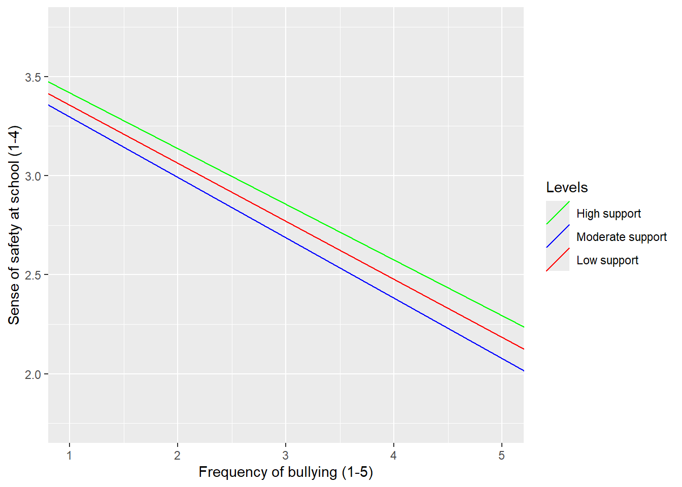
Figure 4: Predicted sense of safety by frequency of bullying. Lines represent trend at 25th, 50th, and 75th percentiles of support from school adults.
Figure 4 shows these lines of best fit. The non-parallel nature of these lines is subtle, but real. The green line, representing students with higher levels of support from school adults, is also the shallowest; more frequent bullying predicts less sense of safety for these students, but not as much as for others. In contrast, the red line shows the association for students who report low levels of support. For these students the relationship is much greater magnitude and differences in experiences in bullying predict more dramatic differences in sense of safety.
These results are consistent with a hypothesis that support from adults works as a protective factor which moderates the association between bullying and experiencing school as unsafe. If a student feels like adults are supportive of her, bullying might have less of an impact on her sense of safety at school. However, our data don’t enable us to demonstrate that this association is causal.
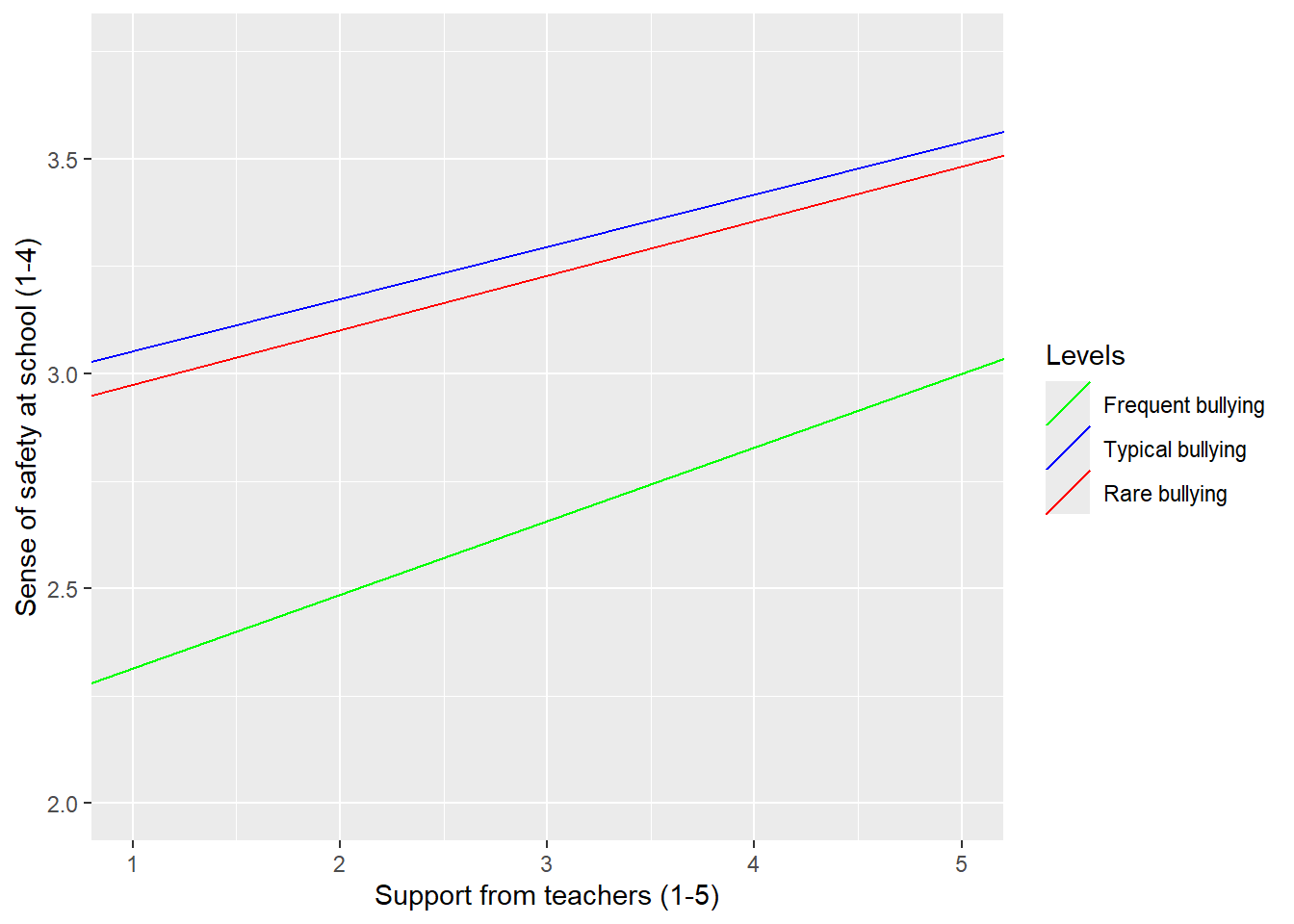
Another way to view these results, which is mathematically equivalent but calls our attention to different features of the relationship, is that the association between support from adults and students’ sense of safety is strongest in students who experience frequent bullying. For students who are not bullied, support from adults is associated with small differences in sense of safety; for students who are bullied frequently, support is associated with much larger differences. We display a plot showing this aspects of the model in Figure 5.
Here we choose the 5th, 50th, and 95th percentiles of the bullying scale as the prototypical values of this variable. These correspond to scale scores of 1 (no bullying), 1.22 (almost no bullying), and 3.11 (fairly frequent bullying). This illustrates the skewed nature of the BULLY variable; most students report no bullying or very little bullying, but a handful of students report extremely frequent bullying. Since the gaps between these prototypical values are not constant, the upper and lower lines are not symmetric about the center line.
Figure 5: Predicted sense of safety by frequency of bullying. Lines represent trend at 25th, 50th, and 75th percentiles of support from school adults.
We would decide how to frame this result depending on which way made more sense to us in the context of our research question.
Code
dat$SAFETY <- dat$safe_scaledat$SUPPORT <- dat$support_scaledat$BULLY <- dat$bully_scaledat$BULLYxSUPPORT <- dat$BULLY * dat$SUPPORTm1 <-lm(SAFETY ~ BULLY, data = dat)m2 <-lm(SAFETY ~ SUPPORT, data = dat)m3 <-lm(SAFETY ~ BULLY + SUPPORT, data = dat)m4 <-lm(SAFETY ~ BULLY + SUPPORT + BULLYxSUPPORT, data = dat)htmlreg(list(m1, m2, m3, m4), ci.force=TRUE)
Table 2: Statistical models predicting sense of safety at school.
Statistical models
Model 1
Model 2
Model 3
Model 4
(Intercept)
3.67*
2.66*
3.18*
3.31*
[ 3.64; 3.70]
[2.60; 2.71]
[ 3.12; 3.24]
[ 3.21; 3.41]
BULLY
-0.31*
-0.30*
-0.38*
[-0.33; -0.29]
[-0.32; -0.28]
[-0.43; -0.32]
SUPPORT
0.16*
0.14*
0.10*
[0.14; 0.17]
[ 0.12; 0.15]
[ 0.07; 0.13]
BULLYxSUPPORT
0.02*
[ 0.01; 0.04]
R2
0.12
0.05
0.16
0.16
Adj. R2
0.12
0.05
0.16
0.16
Num. obs.
7798
7718
7620
7620
* Null hypothesis value outside the confidence interval.
Table 2 displays all of the fitted models predicting students’ sense of safety at school. We prefer Model 4.
Appendix
Other interactions
Multiplying two predictors together is not the only way that we can allow associations to differ according to values of a different predictor. To begin with, interactions involving more than two predictors are also possible; we could create a three-way interaction by taking the product of three different predictors. Additionally, there’s no end of ways that we can combine predictors. For example, we might be interested in regressing SAFETY on BULLY/SUPPORT or BULLY^{SUPPORT} or \sin(BULLY\times SUPPORT). These would make for some bizarre models, but there’s no theoretical reason we couldn’t estimate them. Ideally, your models will be driven by your research questions, theoretical results in your field, and interpretability.
Issues of scale
Quadratic terms and interactions of continuous predictors are frequently on very different scales than the other predictors. For example, in the regression of EMPATHY on GRADE and GRADE^2, the predictor GRADE runs from 6 to 12 while GRADE^2 runs from 36 to 144. The difference between an 11th grader and a 12th grader is a one-unit difference for GRADE, but a 23-unit difference for GRADE^2. So a small regression coefficient for GRADE^2 doesn’t mean that GRADE^2 doesn’t have a strong association with the outcome, it only means that the scale of GRADE^2 is so large that even a tiny regression coefficient indicates a strong association.
The same is true for interactions between continuous variables. Generally the product of two continuous variables is on an extremely large scale. Imagine, for example, interacting IQ with an SES measure that ran from -3 to 3. The interaction would be on a scale of something like -400 to 400 (assuming IQ has a max of around 130). As a result, even in the presence of a strong interaction between SES and IQ, we would expect the estimated regression coefficient to be extremely small, because regression coefficients are scale-dependent.
Plots can make interpretations on coefficients on drastically different (and poorly understood) scales much easier, and should be used whenever possible.
Collinearity
Collinearity is always a potential issue in multiple regression, because we’re frequently interested in controlling for correlated predictors. This is especially true when we’re working with interactions, and even more so when the variables participating in the interactions are continuous. Interactions are almost always highly correlated with the participating variables. Consider the interaction between MALE and GRADE from the running example. For girls there’s no correlation between GRADE and MALE\times GRADE because all girls have a value of 0 for the interaction. However, for boys there is a perfect correlation between the two variables. Even worse, there’s an extremely strong correlation between MALE and MALE\times GRADE. As a result, estimates of the regression coefficients for these variables tend to be very imprecise. Interactions are fun to find, if challenging to interpret, but they can make model-fitting challenging. As a result, it’s best to
test for interactions only when they’re theoretically motivated (which is often true!);
retain them in your model only if they’re statistically significant; and
be careful to distinguish between not finding an association and an association not existing in the population.
We should always be careful of that last point; failure to find convincing evidence of an association does not mean that there is no association in the population. This is especially true when regressing on highly correlated predictors such as interactions and the participating variables. In our experience, researchers frequently think that a null-finding indicates that the population association is 0, but this is a mistake. Remember: to get a sense of the range of plausible population values, look at the confidence intervals. If they’re extremely wide, as they often are when dealing with interactions, it’s hard to say much of anything about the population association.
Centering the predictor
One source of collinearity in models with quadratic terms is the strong correlation between the linear term and the quadratic. Students with a high value of GRADE also have a high value of GRADE^2. This can make it very difficult to estimate the coefficients of each variable, resulting in wide confidence intervals and high p-values. However, there’s an easy fix.10 Take the variable that you want to make quadratic and center it by subtracting the mean from each observation. In the example we used above, we would take
GRADE_i^{ctd} = GRADE_i - \bar{GRADE}_i
Then square these centered values of the predictor to obtain the quadratic variable. The quadratic variable won’t be centered; all of the values will be positive. However, it will be perfectly uncorrelated with GRADE^{ctd}. As a result, standard errors for the coefficients of GRADE^{ctd} and GRADE^{ctd,2} will be much lower, confidence intervals will be narrower, and our estimates will be more precise. Interpretations will be basically unchanged, except the intercept will now be estimating the mean value of the outcome at the mean of the quadratic predictor, rather than when the predictor is 0. This is, typically, a much more interesting concept, which is another advantage to mean centering.
Dropping terms from a model
Some analysts prefer to drop non-statistically significant terms from models. This will usually make our estimates of the remaining terms more precise, which is a good thing. Other analysts suggest that we should keep all of the terms in the model. This will guarantee that our p-values and confidence intervals work as intended. Quadratic terms and interactions make these decisions a little more straightforward.
When fitting a model with a quadratic term, if the quadratic term is not significant, we strongly suggest that you drop it from the model. The presence of a quadratic term drastically complicates the interpretation of the linear term, so we should only retain it if we’re confident that it’s non-zero in the population. However, if the linear term is not statistically significant but the quadratic term is, then we strongly suggest that you retain both terms. Having a linear term doesn’t really make interpretation any more challenging; the quadratic term has already done that. On the other hand, a model with a quadratic term but no linear term is constrained to have an extremum (either a minimum or a maximum) where the quadratic term is equal to 0. This seems like an unreasonable constraint, so we prefer to always include a linear term when we have a quadratic.
We have similar advice for interactions. If you include an interaction in your model, include all of the participating variables. Failing to do so results in a highly inflexible model, which makes too many unjustifiable assumptions.
Common misconceptions
Here are some common misconceptions that you may have
Two predictors are highly correlated, so they must interact. Nope, nope, nope. An interaction occurs when the way a predictor associates with the outcome differs according to the value of another predictor. This says nothing about how the predictors are related with each other. In fact, if two predictors are highly correlated, it might be almost impossible to detect an interaction, even if one exists.
Footnotes
Actually, examining developmental trajectories means measuring students at multiple time points using longitudinal data. These analyses require methods beyond the ones covered in this class. S-052 covers some of the basic techniques. Instead, we’re going to use cross-sectional data to estimate whether there’s an association between grade and self-reported empathic concern across all students. Each student appears only once, but we have students from a range of different grades.↩︎
A monotonic function or association is one in which higher values of x are always associated with higher values of y or are always associated with lower values of y. A monotonic association does not need to be linear, but it’s unidirectional.↩︎
There is no grade 0, so this is not a sensible thing. Equally important, our data only extend from grades six through 12, so it’s incredibly unwise to extrapolate back into elementary school. And let me tell you, I know some elementary schoolers and they are not always super empathic.↩︎
9th graders don’t care very much about each other? Who knew! But that’s also unfair, because the association between grade and empathic concern is incredibly weak and is completely swamped by individual variability. What do you have against 9th graders, you jerk?↩︎
It’s worth pointing out again that this only describes general trends; there are many girls who express low levels of empathic concern and many boys who express high levels.↩︎
The coefficients for the square of grade are really small. That frequently happens when works with square terms. This is not because the quadratic term doesn’t matter as much, it’s because GRADE^2 has a very wide range (from 36 to 144), and when we multiply those big numbers by the very small coefficient, we get moderately large differences. It’s very rare that the magnitude of a regression coefficient is at all meaningful, unless we know both the scale of the predictor and the scale of the outcome.↩︎
Remember, it’s fine to use causal language in deciding what models to fit, but causal associations can’t be inferred from survey data.↩︎
This is arbitrary, and we could also have selected BULLY; the variable which is more germane to the research question should be on the x-axis.↩︎
Remember, we choose prototypical values to be representative/prototypical of the data. Choosing these quartiles shows us students who report moderately low, typical, and moderately high levels of support from their teachers.↩︎
This is a statistical free lunch, if you will. Statisticians sit around centering their variables and thinking how lucky they are.↩︎