This is an addition to the course text where I’ll take you through a brief analysis showing how we could use the tools discussed in class to address an actual research question. I’ll show the necessary code in R and possibly in Stata as well. If there are other things you want to see, please let me know! I will assume that you’ve already read the unit chapter, or at least that you understand the concepts, and will not spend a lot of time reexplaining things.
I’ll try to use data which are publicly available so that you can reproduce the results I share here.
Dataset
For this analysis, I’ll be using data from Project Implicit. Project Implicit runs the Implicit Association Test, or IAT. This test is intended to determine people’s implicit bias, i.e., bias that they may not be willing to express, and may not even know that they hold. The best known version of the IAT is the black-white IAT, which looks for implicit bias against Black or White people. I’ll use data from Project Implicit in Unit 2 when I’ll explain how the test works. One thing to keep in mind is that the people in this sample have chosen to participate in the IAT, and specifically in this version of the IAT. These results may not generalize to the US as a whole.
In this particular application, I’ll be looking at the Transgender IAT which looks for implicit bias against (or, in theory, in favor of) transgender people. On this index, a value of 0 indicates no bias, a positive value indicates a bias against trans people, and a negative value indicates a bias in favor of trans people.
To start with, I need to read in the data. Below you can find the code to do this in R (Stata users, if you want this translated into Stata, please let me know). If you want access to the dataset, let me know and I’ll tell you how to.
Code
library(haven) # this is a package for reading in datasets saved by other statistical packages including SPSSiat <-read_sav('Transgender IAT.public.2023.sav') # you need to make sure that you've set the working directory to be the location where the dataset is saved
Research Questions
I’m going to be asking a few fairly simple questions: what is the distribution of implicit bias against (or in favor of) trans people? Are people who routinely have friendly interactions with trans people less biased against trans people? And finally, is there an association between educational attainment or age and bias against trans people (this is two separate questions).
I expect that, on average, people will demonstrate implicit bias against trans people; certainly there seems to be a great deal of explicit bias against people who are trans, and I hypothesize that the same will be true of implicit bias. I also hypothesize that people who routinely have friendly interactions with trans people will have lower implicit bias; in other contexts it seems that contact reduces implicit bias and I think that will also be true here. And finally, I don’t have a hypothesis about how age or education are associated with implicit bias against trans people.
Analysis
I’m going to take a few steps as a part of this analysis.
Variable Creation
For starters, some of the variables have irritating names that I want to simplify. I also need to create a numeric version of age and label a variable. I’ll do that now.
Code
library(dplyr)library(tidyr)iat <- iat %>%rename(friendly = contacttrans3, bias = D_biep.Cisgender_Good_all)iat$age <-2023- iat$birthyear # this was conducted in 2023, so I'll approximate age as 2023 - birth yeariat$friendly <-recode(iat$friendly, '1'='No', '2'='Yes')iat <- iat %>%drop_na(bias, friendly, age, edu_14) # for this analysis I only want to use people who responded to all four variables that I'm using in my analysis. I lost a lot of people, and I think that's mostly because not everyone is asked the "friendly" itemiat <- iat %>%filter(age >=18, age <=100) # I'm also only keeping people who are between 18 and 100 years old, since the other ages looked unrealistic
Univariate Statistics
Next, I’m going to get some descriptive statistics for the anti-trans implicit bias.
Code
summary(iat$bias)
   Min. 1st Qu.  Median    Mean 3rd Qu.    Max.
-1.8550 -0.1792  0.1487  0.1251  0.4446  1.7928
Code
sd(iat$bias)
[1] 0.4529442
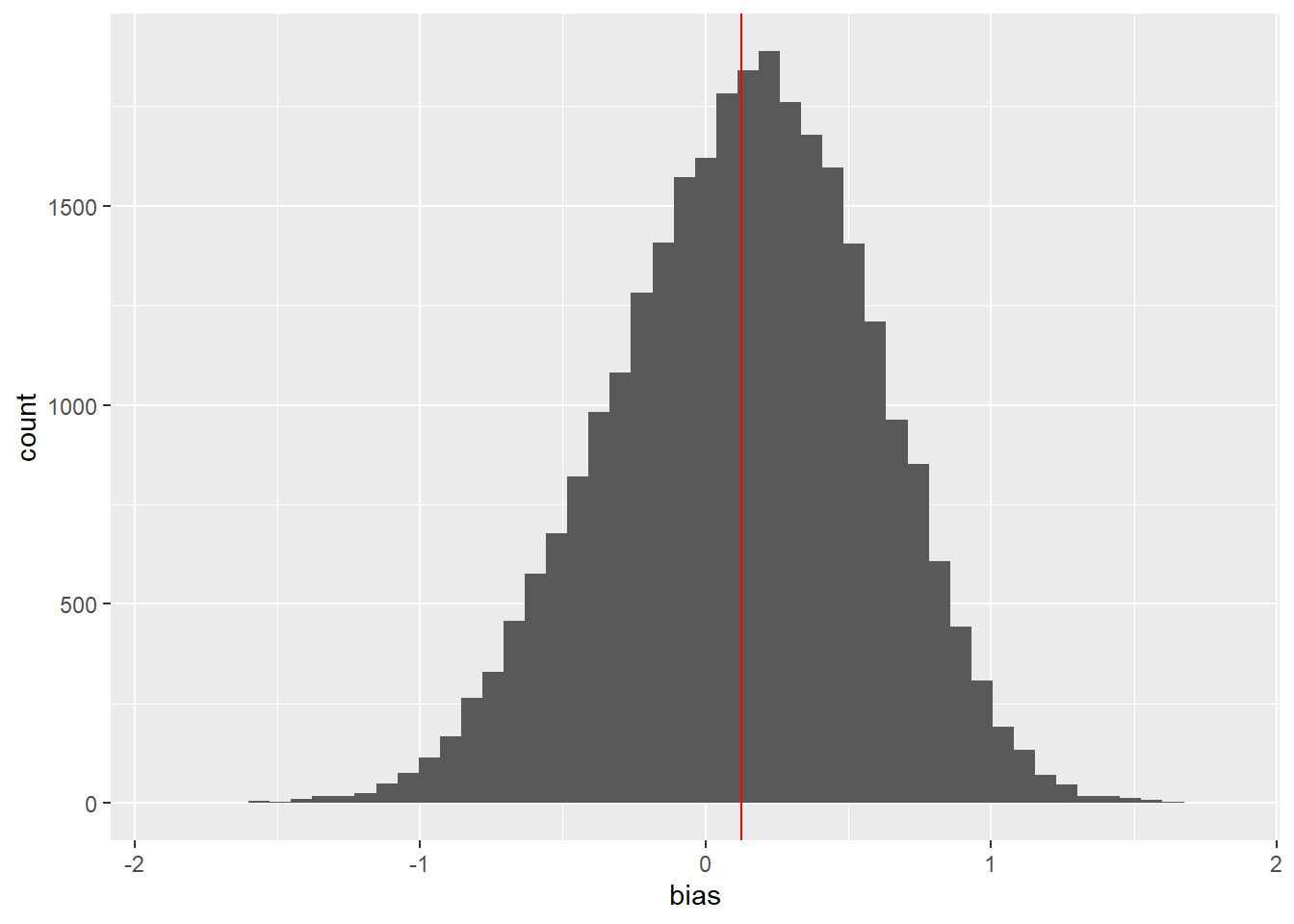
There are a total of 28,402 participants in the dataset. In this sample, the mean respondent had a bias of 0.13 against trans people. It’s a little hard to make sense of this number, but there are some things I can say. First, the value is greater than 0, which indicates that, consistent with my hypothesis, the average respondent has bias against trans people. Second, this bias is smaller than the bias that the average American holds against Black people. Third, given that the standard deviation is 0.45, this is roughly one-third of a standard deviation above 0 (which represents no bias), which I would typically consider a fairly substantial difference. The median bias is 0.15, which is similar to the mean. The central half of the IAT scores fall between -0.18 (which indicates bias in favor of trans people) and 0.44 (which indicates substantial bias against trans people).
Code
library(ggplot2)iat %>%ggplot(aes(x = bias)) +geom_histogram(bins =50) +geom_vline(aes(xintercept =mean(bias)), color ='red')
Here’s a histogram of IAT scores with a vertical red line at the sample mean. The distribution of IAT scores is bell-shaped with a single mode around 0.15. There is a slight negative skew but it is approximately symmetric.
T-Tests
Now I’m going to use a t-test to see if there are differences in mean implicit bias between people who do and do not have regular friendly interactions with trans people.
    Welch Two Sample t-test

data:  bias by friendly
t = 39.005, df = 28366, p-value < 2.2e-16
alternative hypothesis: true difference in means between group No and group Yes is not equal to 0
95 percent confidence interval:
 0.1938647 0.2143795
sample estimates:
 mean in group No mean in group Yes
       0.22855451        0.02443239
About half of the respondents report having regular friendly interactions with a trans person (the exact question is “Do you have friendly interactions with transgender people on a regular basis?”). Keep in mind that these respondents have decided to participate in this test, and this may not reflect the population of the United States, or the world as a whole. It’s also not clear what respondents mean by “friendly interactions” or “on a regular basis”.
However, keeping in mind these limitations, I found a notable difference in implicit bias between people who report having regular friendly interactions and those who do not. The mean implicit bias for people who do not report these interactions is 0.23, so substantially higher than the average. In contrast, people who report regular friendly contact have a mean implicit bias of only 0.02, which is essentially no bias at all. I have compelling evidence that this difference is not just due to chance and that there is a mean difference in a wider population (t(df = 28,366) = 39.00, p < .001), although again, it’s not clear what the wider population really is.
Scatterplots
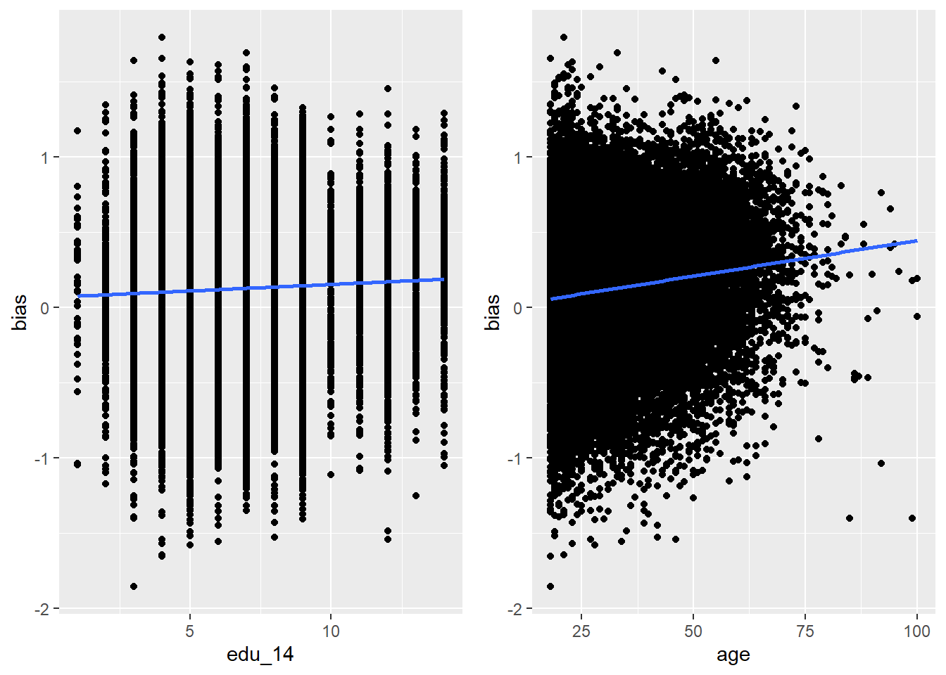
Next, I’m going to look at the association between educational attainment (measured on a 14 point scale) and age and bias against trans people. I’m going to start by looking at scatterplots.
Code
library(gridExtra) # this is for combining the plotsp1 <- iat %>%ggplot(aes(x = edu_14, y = bias)) +geom_point() +geom_smooth(se =FALSE, method ='lm')p2 <- iat %>%ggplot(aes(x = age, y = bias)) +geom_point() +geom_smooth(se =FALSE, method ='lm')grid.arrange(p1, p2, ncol =2)
As often happens with real data, the plots are a little messy. However, there are a few things we can say. First, older people and people with higher levels of education both tend to have higher implicit bias (we’ll quantify that with a correlation next). Second, there’s a tremendous amount of individual variability; at any age and level of educational attainment there’s a huge range of implicit bias. Part of this is because the test is not super accurate, but another part is that people are different from each other, and knowing a person’s age or level of education only tells us a little bit about their implicit bias against trans people.
The association in the age scatterplot (bias scattered on age) might have been strong enough to detect even without the line of best fit overlaid (we’ll discuss this more in unit 3), but I think there’s no way we would have detected it in the education scatterplot.
Correlations and significance tests
Now I want to quantify the strength of the association between bias and each variable, and to test to see if these correlations are difference from 0 in whatever wider population they’re drawn from.
Code
iat %>%cor.test(~ bias + age, .)
    Pearson's product-moment correlation

data:  bias and age
t = 22.718, df = 28400, p-value < 2.2e-16
alternative hypothesis: true correlation is not equal to 0
95 percent confidence interval:
 0.1221584 0.1450032
sample estimates:
      cor
0.1335985
Code
iat %>%cor.test(~ bias + edu_14, .)
    Pearson's product-moment correlation

data:  bias and edu_14
t = 7.4887, df = 28400, p-value = 7.159e-14
alternative hypothesis: true correlation is not equal to 0
95 percent confidence interval:
 0.03278034 0.05599436
sample estimates:
       cor
0.04439334
As we saw in the plots, the association between age and bias (\hat{\rho} = .13) is stronger than the association between education and bias (\hat{\rho} = .04). Both of these are weak correlations, and a correlation of .04 is so small as to be almost undetectable. However, as we often find in big datasets both of these associations are statistically significant. In both cases we’re testing a null-hypothesis that \rho = 0. When looking at age and bias, we reject the null-hypothesis (t(df = 28,400) = 22.7, p < .001), and this is also true when looking at education and bias (t(df = 28,400) = 7.5, p < .001). With this many datapoint, if the null hypothesis were true and there were no linear association between the variables in the “population”, it would be almost impossible to take a sample with a correlation of .04 even though this isn’t a big number from a substantive perspective.
Limitations
In addition to reporting what we found, we want to be clear on what we haven’t found. This is useful both for our audience and for our own understanding.
Here are a few limitations to our analysis. First, none of the associations we measured are necessarily causal. Although it’s tempting to think that regular friendly contact with trans people would lower implicit bias, it’s also possible that people who have lower bias are more comfortable around trans people, leading to more friendly contacts. Second, we always need to keep in mind who was in the sample. These are people who sought out the IAT, and may be quite different from people who would not. Third, we should keep in mind that age and education are correlated with each other. It’s possible that the reason there’s a correlation between education and bias is because highly educated people tend to be older. And fourth, we should make sure to familiarize ourselves with the instrument (the IAT) before interpreting these results, since this will inform how we make sense of our findings.
What’s next?
What’s missing from this analysis? What else would you like to learn about? Send an e-mail to joseph_mcintyre@gse.harvard.edu if you have questions or suggestions!