Unit 3 - Worked example

This is an addition to the course text where I’ll take you through a brief analysis showing how we could use the tools discussed in class to address an actual research question. I’ll show the necessary code in R and possibly in Stata as well. If there are other things you want to see, please let me know! I will assume that you’ve already read the unit chapter, or at least that you understand the concepts, and will not spend a lot of time reexplaining things.

I’ll try to use data which are publicly available so that you can reproduce the results I share here.

Dataset

For this analysis, I’ll be using data from the American Time Use Survey, or ATUS. The ATUS is a product of the Bureau of Labor Statistics (BLS) which measures how Americans spend their time. The ATUS takes a sample of Americans from all over the country, and the results should generalize to all residents of the United States over the age of 15, although there are other time use surveys from other countries. These data include observations from 2003 to 2022.

On the ATUS, people are asked to keep a daily diary for one day. They record their activities as precisely as they can, noting exactly when they began and finished each activity, and then the people who run the ATUS turn their reports into detailed codes. When I say detailed, I mean really, really detailed. For example, there’s one code for “participated in rodeo competitions” and another for “watched rodeo competitions”. There’s another code for “waiting associated with purchasing/selling real estate”. So if you want to understand if Americans are spending more time waiting while purchasing or selling real estate these days than they have in the past, this is the dataset for you. I’m going to be using a slightly simpler version which has compressed some of those very specific codes into something a little more general. Note that the ATUS overrepresents the weekends, so our results are going to be a little skewed.

To start with, I need to read in the data. Below you can find the code to do this in R (Stata users, if you want this translated into Stata, please let me know). If you want access to the dataset, let me know and I’ll tell you how to.

library(readstata13) # this is a package for reading in modern Stata datasets
atus <- read.dta13('atus_sub.dta') # you need to make sure that you've set the working directory to be the location where the dataset is saved

Research Questions

I’m interested in knowing how time spent sleeping has changed over the previous two decades. I hear a lot about how people are getting less and less sleep, and I want to see if that’s born out by the data. More precisely, I want to estimate how much sleep the average American got in 2003, and how much that changed per year over the following two decades.

My hunch, I won’t dignify it by calling it a hypothesis, is that, in fact, people have been getting less sleep over time. As someone who had just graduated college in 2003, I can report that there was nothing to do other than sleep back then. Nowadays there’s a lot more to do, and I think that probably eats into sleep time. I’m also going to see what the association is separately for people with and without a college degree.

Analysis

I’m going to take a few steps as a part of this analysis.

Variable Creation

First off, I know I’m going to be using a linear regression model, regressing time spent sleeping on the year. Since I want to know what the average time spent sleeping was in 2003, and since the intercept represents the mean value of the outcome (time spent sleeping) when the predictor is 0, it would be handy for me to take a variable measuring the year where 0 represents 2003. I’m going to do that by taking year - 2003.

library(dplyr)
library(tidyr)

atus <- atus %>% drop_na(year, time_sleep) # the ATUS is a very well-maintained survey, so this doesn't actually drop anyone.

atus$time_sleep <- atus$time_sleep / 60 # I would rather measure sleep in hours, not minutes

atus$year_cent <- atus$year - 2003 # this will measure the number of years the have elapsed since 2003, so a value of 0 will represent 2003 and, e.g., a 20 would be 2023.

Univariate Statistics

Next, I’m going to get some descriptive statistics for the sleep time.

summary(atus$time_sleep)

   Min. 1st Qu.  Median    Mean 3rd Qu.    Max. 
  0.000   7.500   8.583   8.782  10.000  23.933 

sd(atus$time_sleep)

[1] 2.270871

There are a total of 236,591 participants on the test. In this sample, the mean respondent slept an average of 8.8 hours. Given the scale on which the variable is measured (hours spent sleeping), we can actually make sense of the number. Good for the average respondent, that sounds lovely!¹ There’s a fair spread of sleep time, with the central 50% of respondents reporting between 7.5 and 10 hours of sleep, and a standard deviation of 2.27 hours. Some people report dramatically different amounts of sleep, as low as 0 hours and as high as almost 24 hours.

library(ggplot2)

atus %>% ggplot(aes(x = time_sleep)) + geom_histogram(breaks = seq(0, 24, .25)) + xlim(0, 24) +
  geom_vline(aes(xintercept = mean(time_sleep)), color = 'red')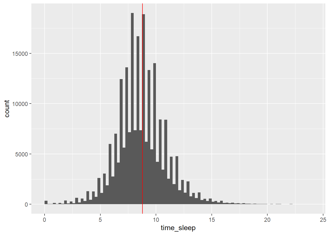

Here’s a histogram of reported time sleeping with a vertical red line at the sample mean. The weird spikes are due people being more likely to report 30 minute increments of sleep; each bin is 15 minutes wide, and we’re probably seeing that people are estimating the amount of time spent sleeping rather than reporting the exact value. Despite that, there seems to be a single mode between 7 and 9 hours of sleep. Notice the right skew; that’s because the maximum amount of time a person can spend sleeping is much further from the mean than the lowest is.

Scatterplot

Now I’m going to scatter sleep time on the year.

atus %>% ggplot(aes(x = year, y = time_sleep)) + geom_point() + geom_smooth(method = 'lm', se = FALSE)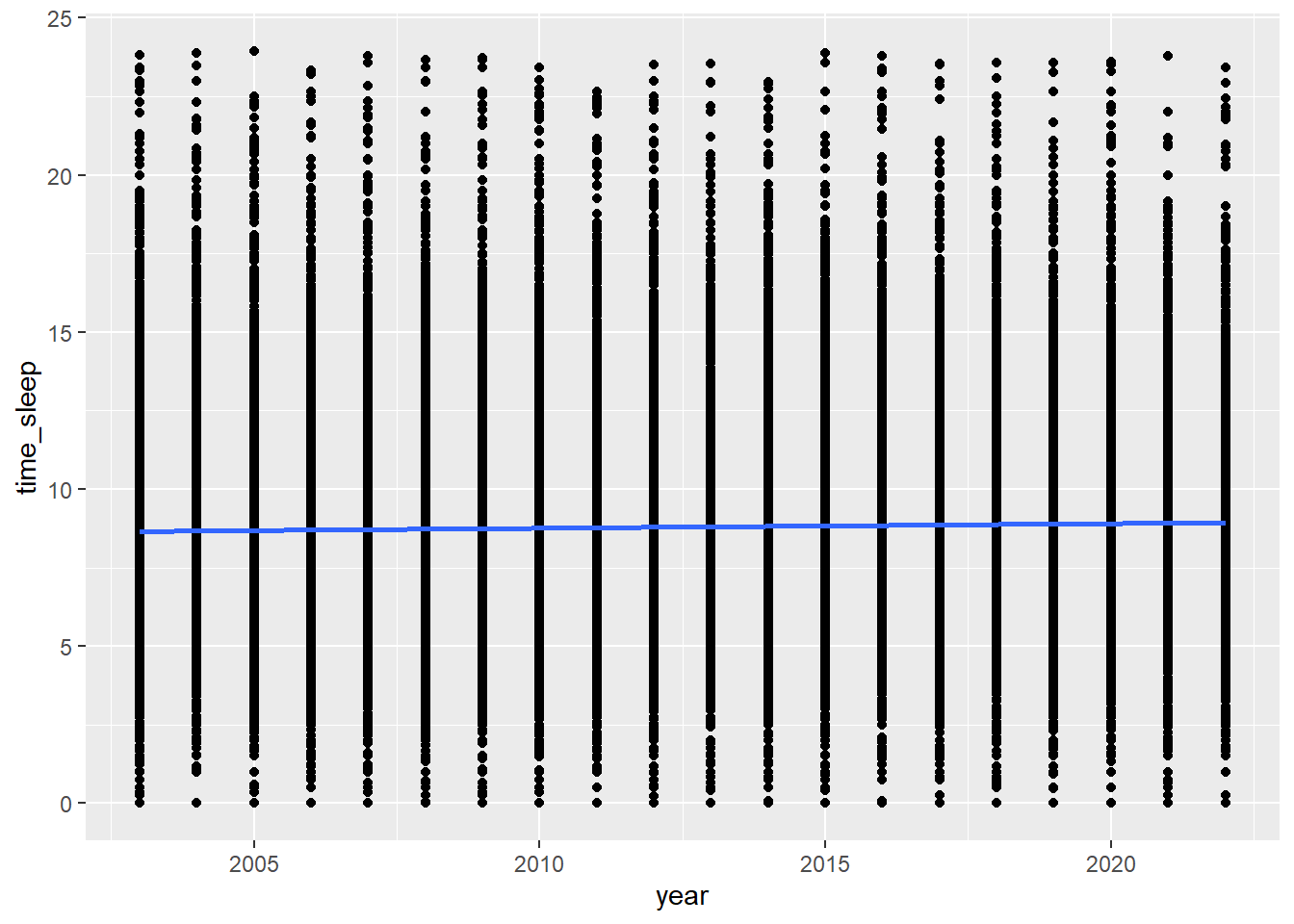

With almost 240,000 observations, it’s hard to see too much in the plot. There’s a hint of a positive association, which is contrary to my “2003 was too boring to stay awake” hypothesis. If I wanted to publish this analysis, I might come up with a new theory that allowed me to claim that I had expected a positive relationship all along. I should also keep in mind that this association is very, very small in magnitude; at a glance it looks like the amount of time spent sleeping hasn’t changed too much.

The Population Model

I’m going to be using a linear regression model to answer my research question, so I should write down a population model. That’s going to look like

time\_sleep_i=\beta_0 + \beta_1year\_cent_i + \varepsilon_i,

where year\_cent is the number of years which have passed since 2003. This is just a generic equation of a line, we’ll use the data to figure out exactly which line fits best. Notice how we use betas and include a residual and how the left-hand side of the equation is the actual outcome.

The fitted model

Now we’ll use our software to figure out which line best captures the association.

library(texreg)
mod <- atus %>% lm(time_sleep ~ year_cent, .)
htmlreg(mod, digits = 3)

Statistical models

	Model 1
(Intercept)	8.659***
	(0.008)
year_cent	0.015***
	(0.001)
R2	0.001
Adj. R2	0.001
Num. obs.	236591
***p < 0.001; **p < 0.01; *p < 0.05

The fitted model is

\hat{time\_sleep_i} = 8.66 + 0.015year\_cent_i

Notice the hat over the outcome, indicating that this is our prediction, the use of actual numbers, and the lack of a residual. Based on my model, I estimate that the average respondent in 2003 got about 8.66 hours of sleep (remember, when year\_cent is 0, the year is 2003). I further estimate that each year Americans reported an additional 0.015 hours (0.9 minutes) of sleep per day, which is counter to my hypothesis. At the same time, the model only explains about 0.1% of the variability in time slept, which means that the vast majority is not explained.

Subsets

Now I’m going to look at things separately for college grads (people with a bachelor’s degree) and non-grads.

mod_coll <- atus %>% filter(educ_simple %in% c('College', 'Grad')) %>% 
  lm(time_sleep ~ year_cent, .)
mod_non_coll <- atus %>% filter(!educ_simple %in% c('College', 'Grad')) %>% 
  lm(time_sleep ~ year_cent, .)
htmlreg(list(mod_coll, mod_non_coll), custom.model.names = c('College', 'Non-college'),
        digits = 4)

Statistical models

	College	Non-college
(Intercept)	8.2861***	8.7993***
	(0.0129)	(0.0105)
year_cent	0.0223***	0.0160***
	(0.0012)	(0.0011)
R2	0.0045	0.0014
Adj. R2	0.0045	0.0014
Num. obs.	78705	157886
***p < 0.001; **p < 0.01; *p < 0.05

Fitting the model separately to subsets consisting of college grads an non-grads, we find that non-grads reported more sleep time in 2003 (8.8 hours v.s. 8.3 hours for college grads), but also gained sleep time more slowly than grads (an additional 0.016 hours per year v.s. 0.022 hours per year for college grads). We won’t have the tools to test to see if this difference is statistically significant for a while.

Limitations

In addition to reporting what we found, we want to be clear on what we haven’t found. This is useful both for our audience and for our own understanding.

Here are a few limitations to our analysis. The key issue is probably that all data are self-reported, and it’s possible that people are not reporting accurately. The BLS works hard to get good data, but getting accurate self-reports is always a challenge. The weird pattern we saw in the histogram suggests that people may be just estimating their sleep time, and it’s possible that that’s causing problems for our analysis. We should also not that we’re assuming that the association between the variables is a straight line, and that may not be correct. We also have not yet tested to see if the associations are statistically significant, so we can’t rule out the possibility that the results are just due to chance. Finally, and this is not really a limitation, we should note that the model doesn’t explain much variability in the outcome. On the other hand, the model estimates that American adults have gained an additional 18 minutes of sleep over the previous 20 years, which is a meaningful amount. Good for us!

What’s next?

What’s missing from this analysis? What else would you like to learn about? Send an e-mail to joseph_mcintyre@gse.harvard.edu if you have questions or suggestions!

Footnotes

1. Jerks.