Unit 4 - Worked example

This is an addition to the course text where I’ll take you through a brief analysis showing how we could use the tools discussed in class to address an actual research question. I’ll show the necessary code in R and possibly in Stata as well. If there are other things you want to see, please let me know! I will assume that you’ve already read the unit chapter, or at least that you understand the concepts, and will not spend a lot of time reexplaining things.

I’ll try to use data which are publicly available so that you can reproduce the results I share here.

Dataset

I don’t do a lot of work with experimental data, so I typically have to track down datasets which have been published by other researchers. This one is from a replication study by some social scientists who were working with the Reproducibility Project. The idea behind the Reproducibility Project is that researchers may find statistically significant effects even when an intervention has no effect just due to chance. Remember, when we set \alpha equal to .05, we accept a 5% chance of incorrectly thinking we’ve found something when nothing has actually happened. This is fine, but it does mean that it’s important to check results before we trust them.¹ Science is supposed to be reproducible, and ensuring that requires scientists to try to reproduce other people’s results. This is especially important since people have a strong incentive to publish results where we reject null-hypotheses and find something, but no real incentive to publish non-findings.

This gives rise to something called the File Drawer Problem. Imagine that 20 people are investigating the same hypothesis, that a particular intervention will have a particular effect. Let’s also assume that in reality the hypothesis is wrong, and there is no effect. Then just by chance, we should expect one of those researchers to find evidence of an association (possibly far more if people engage in p-hacking). Of the 20 original researchers, 19 may find nothing, but lacking any place to publish their results, their papers will end up stashed in some file drawer somewhere. The one person who found something will assume that their results are trustworthy and will publish them. As a result, the scientific literature will suggest that the hypothesis actually was correct, because almost no one will know about all the failed attempts.

That brings us to the Reproducibility Project, which attempted to reproduce a number of papers from cognitive and social psychology. The data we’re working with are an attempt to reproduce a paper called “With a clean conscience: Cleanliness reduces the severity of moral judgments”. The idea behind the initial paper is that moral judgments are tied to our emotional reaction of disgust. We see moral violations as disgusting, just like we might view contact with a filthy object. Consequently, manipulating participants’ sense of physical cleanliness might lead them to change their moral judgments. Specifically, the initial paper found that people who were induced to feel physically clean were less severe in their responses to a series of vignettes asking the respondents to judge someone’s actions. Just to put it simply, people who felt clean were less judgemental.

I’m going to be using data from the replication study, “Does Cleanliness Influence Moral Judgments?”, which used the same procedures with a new group of participants, to see if the results from the initial paper can be reproduced.

To start with, I need to read in the data. Below you can find the code to do this in R (Stata users, if you want this translated into Stata, please let me know). If you want access to the dataset, let me know and I’ll tell you how to.

exp <- read.csv('Exp1_Data.csv') # you need to make sure that you've set the working directory to be the location where the dataset is saved

Research Questions

This analysis will be pretty straightforward. In this experiment, participants were randomly assigned to be primed to think clean thoughts, or to think dirty thoughts (dirty as in “covered with dirt”, not “sexual”). They were then presented with a series of six vignettes describing, e.g., a person who found a wallet on the side of the road and took out all the cash before dropping it.² They were asked to rate each person in terms of the severity We’re going to see if there’s an effect of this random assignment on people’s moral judgments across the vignettes, and then we’re going to see if there was an effect on moral judgments on one particular vignette.

Based on the initial research on this topic, and on the underlying theory, I anticipate that we’ll find evidence that priming people to think clean thoughts will lead them to be less severe in their moral judgments.

Analysis

I’m going to take a few steps as a part of this analysis.

Variable Creation

For starters, I need to label some variables and to create a single variable which represents the average rating that a respondent gave across all the vignettes. This will give me a single “severity” score. I also want to create a dichotomous version of one of the vignettes so I can do a contingency table analysis later. I’m also going to make all of the names lowercase.

library(dplyr)
library(tidyr)

names(exp) <- tolower(names(exp))

exp$condition <- recode(exp$condition, '0' = 'Control', '1' = 'Treatment')
exp$judgment <- exp %>% select(dog, trolley, wallet, plane, resume, kitten) %>% rowMeans()
exp$plane_dich <- cut(exp$plane, breaks = c(-Inf, 4.5, Inf), labels = c('Low', 'High'))

Univariate Statistics

Next, I’m going to get some descriptive statistics for the judgement variables.

exp %>% select(condition) %>% table() %>% prop.table()

condition
  Control Treatment 
0.4885845 0.5114155 

summary(exp$judgment)

   Min. 1st Qu.  Median    Mean 3rd Qu.    Max. 
  2.500   5.833   6.667   6.491   7.167   9.000 

sd(exp$judgment)

[1] 1.12719

exp %>% select(plane_dich) %>% table() %>% prop.table()

plane_dich
      Low      High 
0.1643836 0.8356164 

This experiment involves a total of 219 subjects, with roughly half assigned to treatment and half to control. The average judgment score was about 6.5 on a scale of 0 to 9, indicating that people were fairly severe in their moral judgments for these vignettes. The standard deviation of the judgments was about 1.1. The central half of the responses fell between 5.8 and 7.2.

The specific vignette that we’re going to look at was the plane vignette, where people were told about a group of people involved in a plane crash on an isolated mountain who decide to eat a passenger who was severely injured and certain to die soon.³ People were fairly severe in how they rated the plane vignette, with almost 84% giving a score above the theoretical midpoint of the scale (4.5).

library(ggplot2)

exp %>% ggplot(aes(x = judgment, fill = condition)) + geom_density(alpha = .3)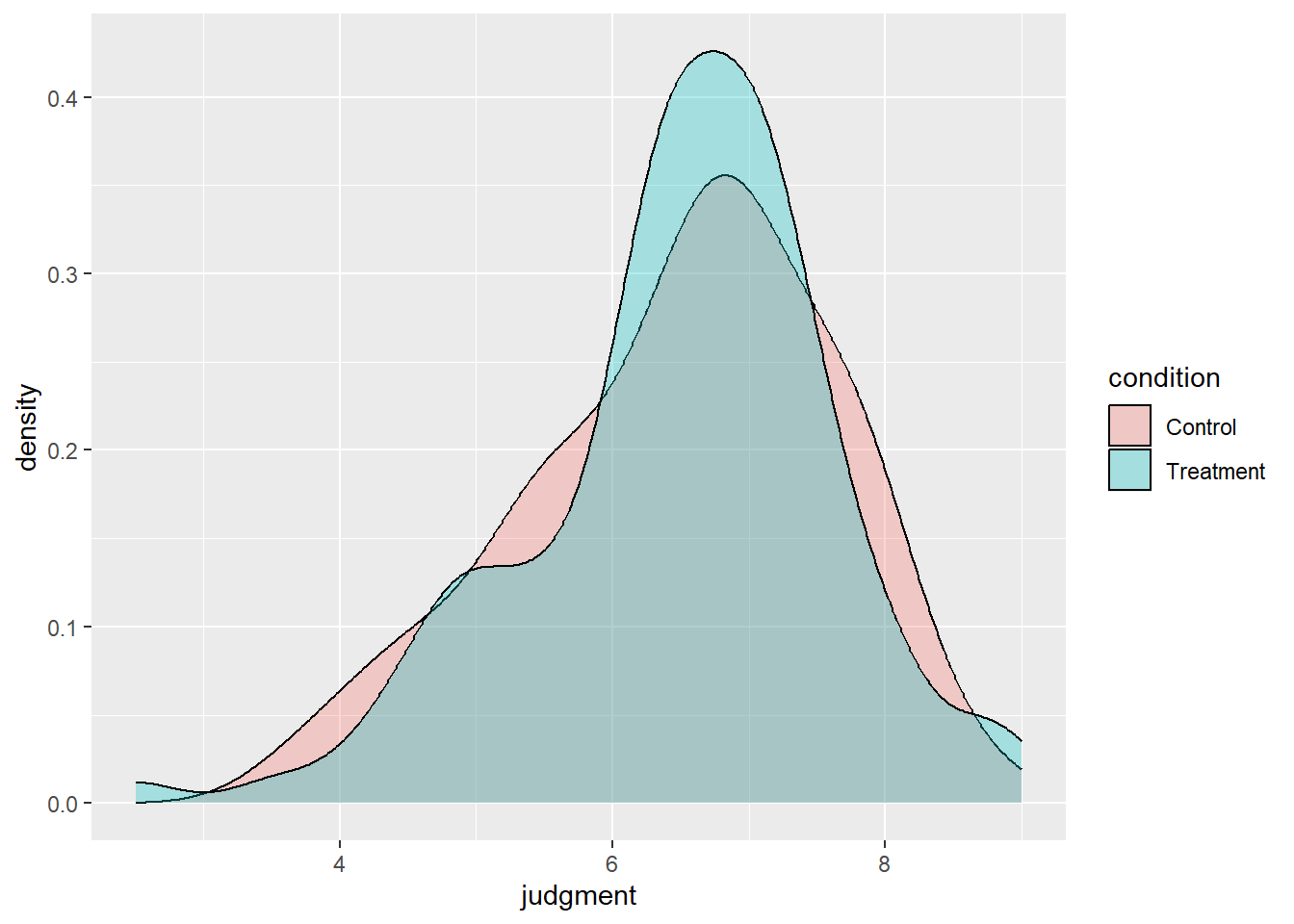

This density plot shows the distribution of judgment separately for people primed to think dirty thoughts (control) and people primed to think clean thoughts (treatment). At a glance, both distributions have a single mode just below 7, have left skews, and look fairly similar to each other, although the control distribution may be a little more spread out. We haven’t done any significance testing yet, but right now it looks like any treatment effect must have been very small.

T-Tests

Now I’m going to use a t-test to see if there’s evidence that the treatment (being primed to think clean thoughts rather than dirty thoughts) impacted the severity of moral judgment (i.e., that the average potential outcome under treatment was more severe than the average potential outcome under control). Remember that a t-test doesn’t not automatically support a causal interpretation, but it does in this case because participants were randomly assigned to treatment v.s. control.

exp %>% t.test(judgment ~ condition, .)

    Welch Two Sample t-test

data:  judgment by condition
t = -0.14226, df = 216.01, p-value = 0.887
alternative hypothesis: true difference in means between group Control and group Treatment is not equal to 0
95 percent confidence interval:
 -0.3229011  0.2794265
sample estimates:
  mean in group Control mean in group Treatment 
               6.479751                6.501488 

Counter to my prediction, the mean severity of moral judgment was actually lower in people assigned to control (6.48) than in people assigned to treatment (6.50). However, the difference was not statistically significant (t(df = 216) = -0.14, p = .887), so there was no evidence that the treatment had an impact at all. More explicitly, if there was no treatment effect, the probability of randomly assigning people to different conditions and obtaining a test statistic this extreme of more is almost 90%.

Contingency Table

Next, I’m going to see if the treatment might have made people more likely to express severe judgments in the plane vignette. This is a fairly artifical thing to do, but I want to practice using contingency tables.

exp %>% select(condition, plane_dich) %>% table() %>% prop.table(margin = 1)

           plane_dich
condition         Low      High
  Control   0.1495327 0.8504673
  Treatment 0.1785714 0.8214286

exp %>% select(condition, plane_dich) %>% table() %>% chisq.test()

    Pearson's Chi-squared test with Yates' continuity correction

data:  .
X-squared = 0.15778, df = 1, p-value = 0.6912

Consistent with our predictions, people primed to think clean thoughts were less likely to judge the actor in the plane incident severely (82%) than were people primed to think dirty thoughts (85%). However, the difference was not statistically significant (\chi^2(df = 1) = 0.16, p = .691), so it’s entirely plausible that this tiny difference could be due to chance.

Limitations

We did not find evidence of a treatment effect on either mean judgment or giving severe judgment on that one item. However, there are a few things to keep in mind. First, the fact that we didn’t find a treatment effect doesn’t mean it wasn’t there. Our results are consistent with no treatment effect, but they’re also consistent with a small treatment effect. We should definitely not claim that we showed that there’s no effect. Second, even if there was no effect in this sample, it would not mean that there was no effect in the initial sample. Remember, treatment effects are sample specific, and there’s no reason the treatment effect should be the same in every sample. And finally, it’s possible that the procedures were different in the two experiments. The team trying to reproduce the results from the first experiment tried to follow the procedures as closely as possible, but it’s possible that they failed to do so.

What’s next?

What’s missing from this analysis? What else would you like to learn about? Send an e-mail to joseph_mcintyre@gse.harvard.edu if you have questions or suggestions!

Footnotes

1. It’s SO important to keep in mind that a researcher need not have done anything wrong to end up reaching an incorrect conclusion. Even when we do everything correctly, there’s a 5% chance of “finding” something that’s not there. That’s why reproduction should not be seen as casting doubt on someone else’s honesty, it’s just a part of the scientific method.

2. There were other vignettes where the moral violation was a little more extravagant.

3. I don’t have the exact text in front of me, and this may not be exactly right. Believe it or not, there were other vignettes where the violations was even more … weird and extreme.