Unit 5 - Worked example

This is an addition to the course text where I’ll take you through a brief analysis showing how we could use the tools discussed in class to address an actual research question. I’ll show the necessary code in R and possibly in Stata as well. If there are other things you want to see, please let me know! I will assume that you’ve already read the unit chapter, or at least that you understand the concepts, and will not spend a lot of time reexplaining things.

I’ll try to use data which are publicly available so that you can reproduce the results I share here.

Dataset

For this analysis, I’ll be using data from the American Community Survey, or ACS. The ACS is a product of the US Census which measures various data about Americans, including financial data. The ACS takes a massive sample of over a million households per year. It’s used for all sorts of purposes, including helping businesses plan where to open new locations and invest, and for academic research. People contacted by the ACS are required by law to respond to the survey which results in high response rates. The population of the ACS is all non-institutionalized adults living in permanent residences in the United States. These data are from 2022 and represent a small subset of all the records available. This is NOT a random subset, and these data cannot be used to represent the whole population, but if you want to work with the full ACS, I can help with that.

To start with, I need to read in the data. Below you can find the code to do this in R (Stata users, if you want this translated into Stata, please let me know). If you want access to the dataset, let me know and I’ll tell you how.

library(readstata13) # this is a package for reading in modern Stata datasets
acs <- read.dta13('acs_sub_2022.dta') # you need to make sure that you've set the working directory to be the location where the dataset is saved

Research Questions

I’m interested in knowing how educational attainment is associated with income. In unit 7, we’ll find a better way to look at this, but for now I’m going to look for a linear association between level of schooling (the variable schl records something like years of schooling completed by the respondent) and income (the pincp variable). My hypothesis is that higher levels of education are associated with higher incomes because I expect that completing education increases a person’s income. Note that, although I hypothesize that there’s a causal association here, I won’t be able to demonstrate that from this analysis since there’s no way to identify a causal effect with these data. If there is an association, it could be that both education and income are being caused by some third variable. Maybe people from high income backgrounds have high incomes and high educational attainment.

Analysis

I’m going to take a few steps as a part of this analysis.

Univariate Statistics

First, I’m going to get some descriptive statistics for wages and education.

library(dplyr)
summary(acs$pincp)

   Min. 1st Qu.  Median    Mean 3rd Qu.    Max. 
  -2300   23500   45000   64521   79000 1212000 

sd(acs$pincp)

[1] 80440.36

summary(acs$schl)

   Min. 1st Qu.  Median    Mean 3rd Qu.    Max. 
   1.00   16.00   19.00   18.72   21.00   24.00 

sd(acs$schl)

[1] 3.447581

The average respondent reported income of almost $65,000. The central 50% of respondents earned between $23,000 and $79,000. Some respondents reported negative income, and the highest reported income is $1.2 million (although this may just be the highest value the ACS reports). The median income, $45,000, is substantially lower than the mean, which indicates a right-skewed distribution. The standard deviation of income is also quite large ($80,000), which suggest great variability in incomes.

In contrast, the mean and median levels of schooling are quite close, at around 19 (the units are hard to make sense of here, but this corresponds to one year of college credit but no degree). The standard deviation is 3.44, and the central 50% of respondents fall between 16 (high school diploma) and 21 (a bachelor’s degree).

library(ggplot2)

acs %>% ggplot(aes(x = pincp)) + geom_histogram(bins = 100) + 
  geom_vline(aes(xintercept = median(pincp)), col = 'red')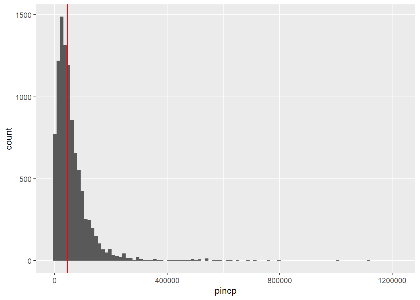

As expected, the distribution of income is severely right-skewed with a single mode somewhere slightly below the median, and an extremely long right tail.

Scatterplot

Now I’m going to scatter income on education.

acs %>% ggplot(aes(x = schl, y = pincp)) + geom_point() + geom_smooth(method = 'lm', se = FALSE)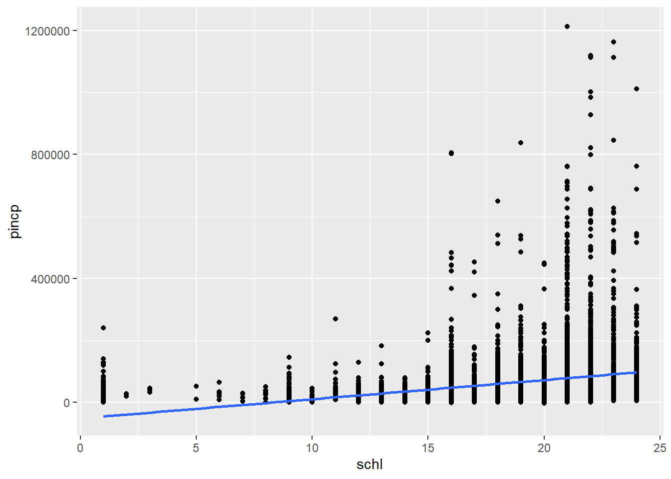

The scatterplot is a little hard to make sense of. There does appear to be a positive association between income and education, although it’s not necessarily linear. There’s a tremendous amount of individual variability, especially at higher levels of education. The line of best fit predicts negative income at low values of education, which does not appear to be realistic. This is a problem with our model which we’ll try to address using new tools in unit 7.

The Population Model

I’m going to be using a linear regression model to answer my research question, so I should write down a population model. That’s going to look like

income_i=\beta_0 + \beta_1schl_i + \varepsilon_i.

Remember, since this is a population model and we don’t know what the actual values of \beta_0 and \beta_1 are, we’ll refer to them with Greek letters. They don’t have hats on them because they’re not our estimates, they’re the actual values in the population, which we happen not to know.

The fitted model

Now we’ll use our software to figure out which line best captures the association.

library(texreg)
mod <- acs %>% lm(pincp ~ schl, .)
htmlreg(mod)

Statistical models

	Model 1
(Intercept)	-51211.62***
	(4283.27)
schl	6181.85***
	(225.01)
R2	0.07
Adj. R2	0.07
Num. obs.	10000
***p < 0.001; **p < 0.01; *p < 0.05

The fitted model is

\hat{pincp_i} = -51212 + 6182schl_i

One silly thing about this model is that it predicts that people with a value of schl of 0 will have an income of less than -$50,000. That’s not realistic. More raesonably, the model predicts that each additional level of schl (something like each additional year of schooling, though not quite) is associated with an additional $6,200 of income. So as we anticipated, at least in our sample, more schooling is associated with higher wages.

The Standard Error

The standard error for the slope estimate is 225 (technically, $225 per additional level of schooling). This is our estimate of the standard deviation of the sampling distribution of the slope estimate across repeated random samples, and gives us a sense of how precisely or imprecisely the slope has been estimated.

T-test

We also use the standard error in conducting a t-test. The t-test is testing a null-hypothesis of no linear association between the outcome and the predictor in the wider population. We could express this as

H_0: \beta_1 = 0

We conduct a t-test by 1) taking the observed value of \hat{\beta_1} (6,182), 2) subtracting the hypothesized value of \beta_1 (0), and dividing by the estimated standard error of the slope (\hat{se}(\hat\beta_1)). This gives us a value of

\frac{6182 - 0}{225} = 27.47

for the t-statistic. Comparing this to a t-distribution with 9,998 degrees of freedom (sample size - 2) gives us a p-value of (substantially) less than .001. We might report this by saying something like “we rejected a null-hypothesis of no linear association between schooling and income (t(df = 9,998) = 27.47, p < .001) and estimated that each level difference in schooling is associated with a roughly $6,000 difference in income, with people with more education outearning people with less education”.

This isn’t the only hypothesis we could test. Let’s say, for example, that economists had determined that it’s only worth pursuing more education if each year is associated with at least $5,000 in additional income. Setting aside the fact that our data don’t allow us to make causal claims, we could test a hypothesis that the slope is equal to 5,000, or

H_0: \beta_1 = 5000

To do that by hand, we would just take

\frac{6182 - 5000}{225} = \frac{1182}{225} \approx 5.25

We could compute the exact p-value (R users, see below), but we can also note that the t-statistic is larger than 2, so p < .05, and furthermore it’s larger than 3.8, so p < .001.

dt(5.25, df = 9998) # this is the proportion of a t-distribution with df = 9,998 which lies ABOVE 5.25. To get the proportion that lies ABOVE 5.25 or BELOW -5.25 (so more extreme than 5.25), we would take

[1] 4.201606e-07

dt(5.25, df = 9998) * 2 # the p-value is about .000000840, which we would write as p < .001.

[1] 8.403212e-07

Confidence Intervals

confint(mod)

                 2.5 %     97.5 %
(Intercept) -59607.690 -42815.543
schl          5740.792   6622.915

While it’s interesting to be able to say that we have evidence that the slope is not equal to 0 or 5000, and is in fact greater than those values, that doesn’t tell us a lot about what the slope IS. However, we can use the idea of t-testing to construct a confidence interval consisting of all the possible values of \beta_1 for which we would fail to reject a hypothesis. That is, all the population values of the slope which are consistent with our sample. We do that by taking the observed slope and going out two estimated standard errors on either side; for any of these values a hypothesis test would result in -2 \le t \le 2, and we would fail to reject the hypothesis. So construct the confidence intervals as roughly

6182\pm2\times225 \approx (5741, 6623)

So we’re 95% confident that the actual slope is somewhere in the range of 5,741 to 6,623, although we can’t be certain, and we don’t know the exact value. But again, if we decided that getting an additional year of schooling would be worth it only if the true association was above 5,000, this should make us confident that the additional schooling is a good idea since all the values in the confidence interval are above that threshold.

Limitations

In addition to reporting what we found, we want to be clear on what we haven’t found. This is useful both for our audience and for our own understanding.

First off, we can’t know for certain that our results are correct. Even if we do everything right, it’s possible to reach incorrect conclusions just by chance. On the other hand, given the p-value, it’s hard to imagine that this is just a chance sample from a null-population. Second, we’re assuming that there’s a linear association between schooling and income, and this seems unlikely. We’ll have to wait until unit 7 to fix this, though. Finally, we can’t say that this is a causal association. It’s certainly possible that additional schooling leads to higher incomes, but these data can’t demonstrate that. It’s also possible, for example, that kids from high socioeconomic backgrounds are more likely to attend school for an extended period of time and also more likely to have high incomes, but there’s no causal association (or more likely that there still is a causal association, it’s just not identical to the one we estimated). Given how our data were collected, it’s unlikely that we’ll be able to construct a counterfactual for what someone’s income would have been if they had more or less education than they actually do, so we may not be able to address causal questions. That’s okay! Not every question needs to be about causal effects!

What’s next?

What’s missing from this analysis? What else would you like to learn about? Send an e-mail to joseph_mcintyre@gse.harvard.edu if you have questions or suggestions!