Code
library(haven)
iat <- read_sav('Transgender IAT.public.2023.sav') # you need to make sure that you've set the working directory to be the location where the dataset is savedThis is an addition to the course text where I’ll take you through a brief analysis showing how we could use the tools discussed in class to address an actual research question. I’ll show the necessary code in R and possibly in Stata as well. If there are other things you want to see, please let me know! I will assume that you’ve already read the unit chapter, or at least that you understand the concepts, and will not spend a lot of time reexplaining things.
I’ll try to use data which are publicly available so that you can reproduce the results I share here.
For this analysis, I’ll be going back to the data from the Transgender IAT. You might want to review the discussion from the Unit 2 worked example, but for now note that 1) scores of 0 indicate no implicit bias against or in favor of trans people (compared to cisgender people), 2) scores above 0 indicate implicit bias against trans people, and 3) scores below 0 indicate implicit bias in favor of trans people.
To start with, I need to read in the data. Below you can find the code to do this in R (Stata users, if you want this translated into Stata, please let me know). If you want access to the dataset, let me know and I’ll tell you how to.
library(haven)
iat <- read_sav('Transgender IAT.public.2023.sav') # you need to make sure that you've set the working directory to be the location where the dataset is savedI’m interested in knowing if there’s an association between political ideology and implicit bias against trans people. There are definite differences in how liberals and conservatives tend to talk about trans people, but it’s not clear that this also reflects implicit bias. It’s possible that there’s no association between implicit bias against trans people and political ideology. I’m not going to look at this on an individual level, though. Instead, I’m going to see if there’s an association between average implicit bias as measured at the Metropolitan Statistical Area (MSA) level (sort of like a city or metro area) and average political leaning. Just to be completely upfront, I’m doing this because I think it will make for a more interesting example of looking at residuals. It’s not an approach I would probably take in reality. If you want to reproduce this analysis at the level of the individual responder, go for it!
I’m going to take a few steps as a part of this analysis.
First off, I need to take the IAT dataset, which is measured at the individual level, and aggregate up to the MSA level, computing the average IAT score and the average political ideology (on a scale of -3 = very conservative to 3 = very liberal; so we’ll think of this as a scale of political liberalism).
library(dplyr)

iat <- iat %>% select(msa = MSAName, iat = D_biep.Cisgender_Good_all, liberal = politicalid_7) %>% # choose the variables I want, rename them, and do the aggregation
  group_by(msa) %>%
  summarize(n = n(), # find the number of observations
            iat = mean(iat, na.rm = TRUE),
            liberal = mean(liberal, na.rm = TRUE) - 4) %>% # liberal was on a scale of 1 to 7, so this just shifts it to -3 to 3
  na.omit() # only keep those MSAs with observed data

iat %>% arrange(liberal) %>% head() # these are the most conservative MSAs
# A tibble: 6 × 4
msa n iat liberal
<chr> <int> <dbl> <dbl>
1 APO 1 0.139 -3
2 Gadsden, AL MSA 3 0.454 -1
3 Texarkana, TX-Texarkana, AR MSA 12 0.0104 -0.75
4 Ocean City, NJ MSA 8 0.270 -0.625
5 Alexandria, LA MSA 13 0.419 -0.615
6 Lebanon, PA MSA 21 0.304 -0.571iat %>% arrange(desc(liberal)) %>% head() # these are the most liberal MSAs# A tibble: 6 × 4
msa n iat liberal
<chr> <int> <dbl> <dbl>
1 Corvalis, OR MSA 81 -0.0627 2.03
2 San German-Cabo Rojo, PR MSA 1 0.872 2
3 Ithaca, NY MSA 62 -0.104 1.84
4 Danville, IL MSA 6 0.0541 1.8
5 Eugene-Springfield, OR MSA 142 -0.0241 1.75
6 Ann Arbor, MI MSA 321 0.0530 1.65I’m not going to do too much of this, but I do want to look at the distribution of IAT scores and liberalism.
library(ggplot2)
iat %>% ggplot(aes(x = iat)) + geom_density() + geom_vline(aes(xintercept = mean(iat)), color = 'red')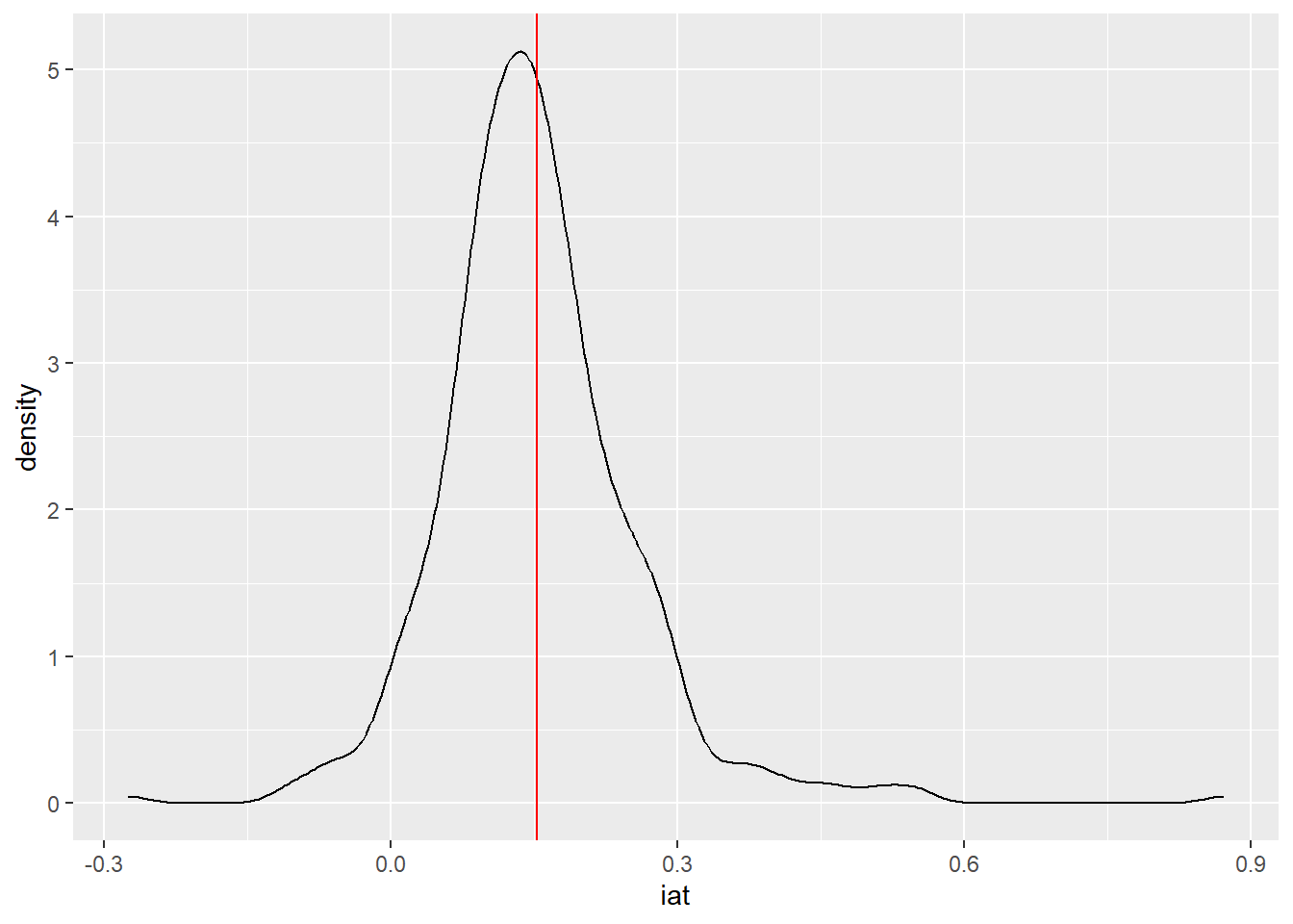
iat %>% ggplot(aes(x = liberal)) + geom_density() + geom_vline(aes(xintercept = mean(liberal)), color = 'red')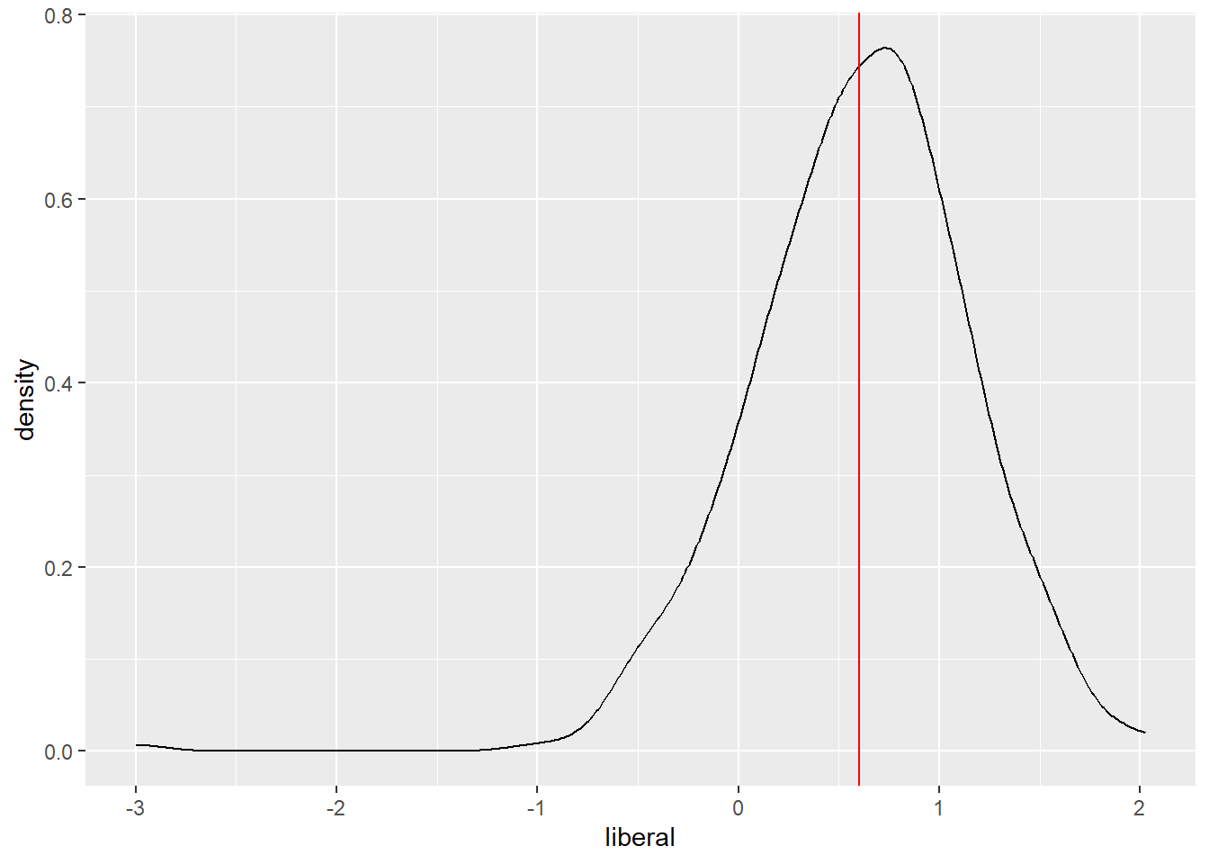
Recall that for both variables, a value of 0 has a special meaning. For IAT scores, 0 indicates no mean bias; for liberalism, 0 indicates that the average political affiliation is moderate. Looking at the distribution of IAT scores, the mean MSA has low bias against trans people, with an IAT score of something like 0.15. The distribution is right skewed, with a handful of MSAs showing slight bias in favor of trans people, and a long right tail of much higher bias against trans people (it looks like the high value might be driven by a single MSA).
The average MSA is slightly liberal, with a score of something like 0.6; this probably says more about who chooses to take this particular version of the IAT than about the distribution of political ideology around the country. There is a single MSA where the one person surveyed reported being very conservative, and a handful of MSAs where the mean response was liberal. The vast majority of MSAs seem to be slightly conservative (-0.5) to somewhat liberal (1.5).
Now I’m going to scatter mean IAT on mean liberalism.
library(plotly) # this will add some interactivity to the plot
(iat %>% ggplot(aes(x = round(liberal, 2), y = round(iat, 2), text = paste0(msa, ': ', n))) + geom_point()) %>%
  ggplotly()
Notice that there does seem to be a negative association between liberalism and IAT scores. MSAs which are more liberal tend, on average, to have less implicit bias against trans people. However, it’s not a perfect association. There’s an MSA, APO (I believe this is a military designation), where the one respondent was extremely conservative but had a relatively moderate level of implicit bias, and that data point may be skewing our results. We’ll keep that in mind for later. There’s also a lot of variability. Despite the general trend, at any level of liberalism there appears to be a wide spread of IAT scores.
I’m going to be using a linear regression model to answer my research question. Here’s the model I’m going to fit:
iat_i=\beta_0 + \beta_1liberal_i + \varepsilon_i,
library(texreg)
mod <- lm(iat ~ liberal, data = iat)
htmlreg(mod)| Model 1 | |
|---|---|
| (Intercept) | 0.20*** |
| (0.01) | |
| liberal | -0.07*** |
| (0.01) | |
| R2 | 0.14 |
| Adj. R2 | 0.14 |
| Num. obs. | 424 |
| ***p < 0.001; **p < 0.01; *p < 0.05 | |
confint(mod) 2.5 % 97.5 %(Intercept) 0.18292732 0.2106741 liberal -0.08993976 -0.0557168
The fitted model is
\hat{iat}_i = 0.20 - 0.07liberal_i
We estimate that in MSAs which are moderate politically (liberal = 0), the mean IAT score will be 0.20, indicating slight implicit bias against trans people. We also estimate that each additional level on the liberalism scale (mean MSAs which are more liberal) is associated with a -0.07 point difference in mean IAT scores. Notice that we estimate that in extremely liberal MSAs, where liberal = 3, IAT will be equal to 0.20 - 3\times0.07 = 0.20 - 0.21 = -0.01, or essentially no bias. However, this is an almost impossibly liberal MSA where every single person identifies themselves as extremely liberal. We’re 95% confident that the true slope falls between -0.09 and -0.06; notice that we can infer that the result is statistically significant. We should also note that the model is only explaining about 14% of the variability in mean IAT scores.
Now I’m going to check the regression assumptions by looking at the distribution of the residuals.
iat$res <- rstandard(mod)
iat %>% ggplot(aes(x = liberal, y = res)) +
  geom_point() +
  geom_smooth(se = FALSE, color = 'red', lty = 2) +
  geom_hline(yintercept = 0)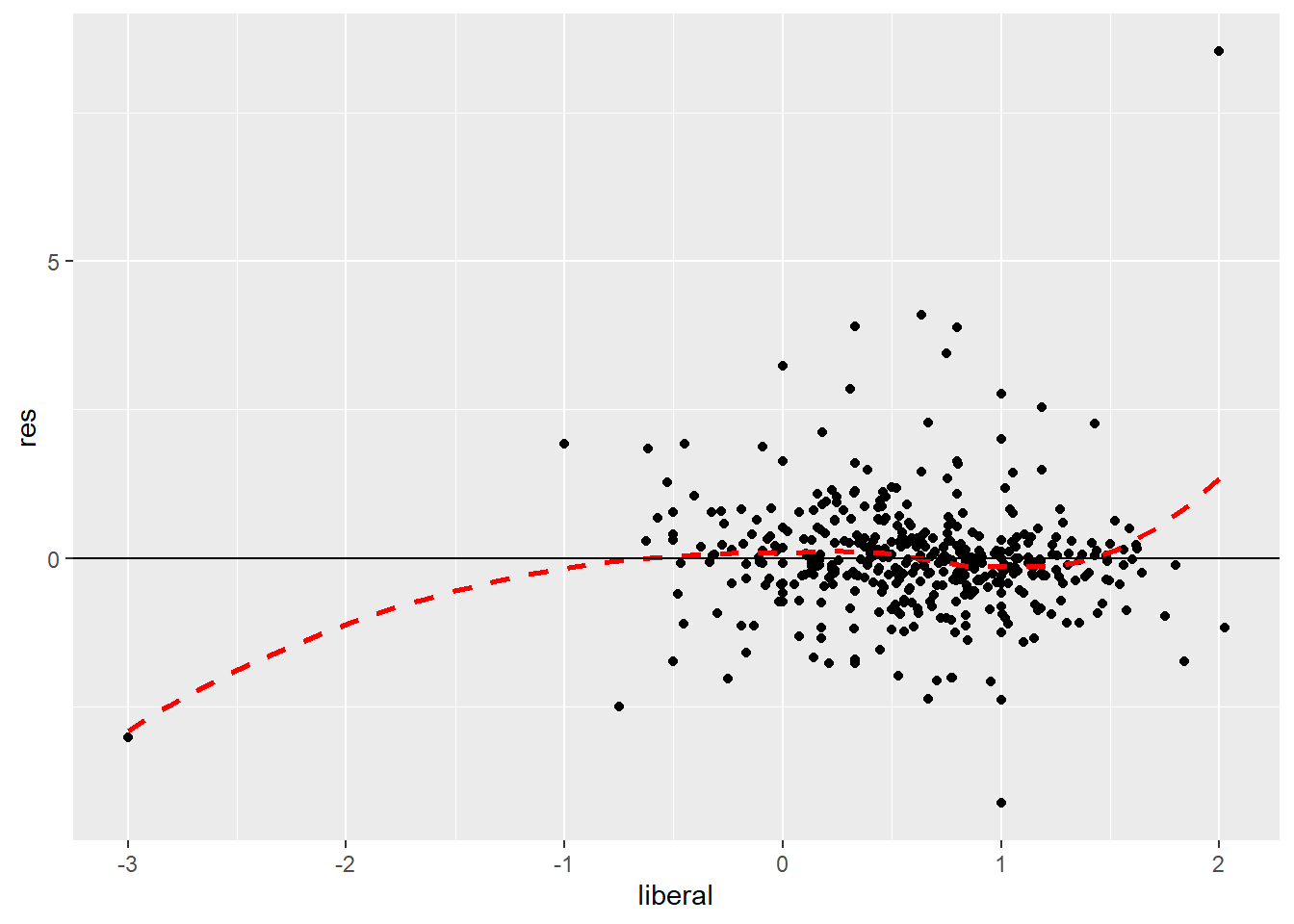
First looking at a scatter of the standardized residuals on liberal, I’ll check the assumptions of linearity and homoscedasticity. That one unusual MSA, the only one which is extremely conservative and has a moderate IAT score, seems to be messing with the LOWESS curve at the far left of the plot. However, focusing on the part of the plot where we actually have data, the LOWESS curve appears to be close to the line y = 0, which suggests that our assumption of linearity is at least plausible (remember, we don’t pay too much attention to what’s happening at the edges of the scatterplot where the LOWESS curve is sensitive to individual observations).
The residuals show approximately equal vertical scatter at each value of the predictor, suggesting that the assumption of homoscedasticity is also plausible.
iat %>% ggplot(aes(x = res)) +
  geom_histogram(aes(y = after_stat(density))) +
  geom_density(se = FALSE, color = 'red', lty = 2) +
  stat_function(fun = dnorm, color = 'blue')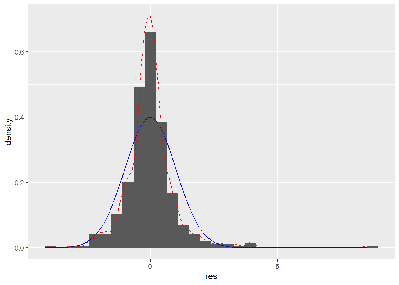
The distribution of the residuals is not Normal. There’s a strong right skew and far too many large residuals for a Normal distribution.
The assumption of Normality is unlikely to matter too much in a large dataset like this. Given that the assumptions of linearity and heteroscedasticity appear at least plausible, we should consider our estimates trustworthy. However, just to be safe I’m going to refit the model, this time only using MSAs where at least 10 people participated in the survey. With very small MSAs, we have so little data on bias and liberalism that we might not want to trust our results.
iat %>% filter(n >= 10) %>%
  lm(iat ~ liberal, .) %>%
htmlreg()| Model 1 | |
|---|---|
| (Intercept) | 0.20*** |
| (0.01) | |
| liberal | -0.09*** |
| (0.01) | |
| R2 | 0.25 |
| Adj. R2 | 0.24 |
| Num. obs. | 400 |
| ***p < 0.001; **p < 0.01; *p < 0.05 | |
Although the fitted model is different after removing those small MSAs, our conclusion that more liberal MSAs tend to have lower bias against trans people remains unchanged.
library(stringr)
iat$raw_res <- residuals(mod)
(iat %>% ggplot(aes(x = round(liberal, 2), y = round(iat, 2), text = paste0(msa, ': ', round(raw_res, 2)))) +
   geom_point() +
   geom_point(data = iat %>% filter(str_detect(msa, 'MA ')), color = 'red')) %>%
  ggplotly()
At this point, it might be interesting to look at individual residuals to find places with unusually high or low levels of implicit bias. I’ve picked out all the Massachusetts MSAs in red. Notice that Worcester, a slightly liberal MSA, has a mean IAT which is about 0.08 higher than expected. It’s not an unusually high IAT, but it’s a little higher than we would have predicted give Worcester’s political leanings. In contrast, the non-metro MA MSA is less liberal than Worcester, but has a much lower mean IAT score. In fact the mean IAT in that MSA is about 0.20 lower than we predicted. Feel free to find other MSAs, and R users, you can edit the code to highlight the MSAs that interest you.
There are a LOT of limitations here. First, as I mentioned earlier, it’s not really clear that we should be looking at this at the MSA level, I did that just to make the residual analysis more interesting. Second, we only have a very rough estimate of the mean liberalism and IAT score in each MSA; some of them only have a single participant which means that we’re basing our estimate of the mean in those MSAs based on what one person put. This is an even bigger issue given how much measurement error is inherent in IAT scores; these are very noisy estimates. We should also note that political affiliation is self-reported. Two people who both call themselves moderate might have very different standards for what that means. And, of course, political beliefs are complex and hard to reduce to a single dimension. Another really important thing to remember is that we’re basing our inferences on people who chose to participate in the IAT. It’s possible that, e.g., there are lots of conservative Americans with extremely low implicit bias who simply didn’t participate in the research by Project Implicit. And finally, as I mention in almost all of these, we can’t draw causal inferences here. These data give us no reason to think that a person’s/MSA’s political leanings impact their implicit bias. Again, this is something we always want to keep in mind, it’s not unique to this analysis, but it’s really important to remember.
What’s missing from this analysis? What else would you like to learn about? Send an e-mail to joseph_mcintyre@gse.harvard.edu if you have questions or suggestions!