Unit 7 - Worked example

This is an addition to the course text where I’ll take you through a brief analysis showing how we could use the tools discussed in class to address an actual research question. I’ll show the necessary code in R and possibly in Stata as well. If there are other things you want to see, please let me know! I will assume that you’ve already read the unit chapter, or at least that you understand the concepts, and will not spend a lot of time reexplaining things.

I’ll try to use data which are publicly available so that you can reproduce the results I share here.

Dataset

For this analysis, I’m going to return to the ACS dataset. Previously we had looked at how educational attainment is associated with income, now we’re going to try to use a log transformation to improve our results. Look at unit 5 for a description of the dataset.

To start with, I need to read in the data. Below you can find the code to do this in R (Stata users, if you want this translated into Stata, please let me know). If you want access to the dataset, let me know and I’ll tell you how.

library(readstata13) # this is a package for reading in modern Stata datasets
acs <- read.dta13('acs_sub_2022.dta') # you need to make sure that you've set the working directory to be the location where the dataset is saved

Research Questions

I’m still interested in knowing how educational attainment is associated with income, but this time we’re going to try log transforming the outcome variable (personal income). As before, we predict that there will be a positive association between income and educational attainment, although even if we find this association there’s no way to demonstrate that the association is causal.

Analysis

I’m going to take a few steps as a part of this analysis.

Filter the dataset

I’m going to be log-transforming the income variable (I’ll explain why later). However, it’s only possible to log-transform positive values. Recall from unit 5 that some people reported negative income. As a result, I need to do something about these folks. There are a few things I could do, but I’m going to just drop anyone with an income of $0 or less. This will change the population I can describe (people with positive income), but it won’t change our dataset too much (we’ve already subsetted to only include people with positive wages to make this dataset more useful in unit 9).

library(dplyr)
acs <- acs %>% filter(pincp > 0)

In fact, we only lost two respondents.

Histogram

To justify a log-transformation, let’s look at the distribution of incomes (below).

library(ggplot2)

acs %>% ggplot(aes(x = pincp)) + geom_histogram(bins = 100) + 
  geom_vline(aes(xintercept = median(pincp)), col = 'red')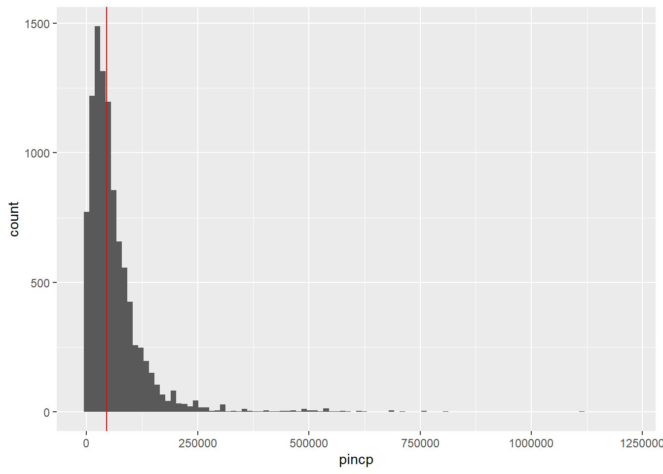

Notice that 1) the distribution is extremely right-skewed, and 2) it only includes positive values. Both of those are signals that we MAY want to log transform the variable (although we’ll need additional information before making that decision). Some other reasons that income may be a good variable to log are that income has a meaningful value of 0 (0 income actually means that a person has no income), and with income, percentage differences may be more meaningful than absolute differences. For example, the difference between an income of $10,000 and $20,000 is much larger in practical terms than the difference between $1,000,000 and $1,010,000, even though in both cases the difference is $10,000.

Scatterplot

Now I’m going to scatter income on education.

acs %>% ggplot(aes(x = schl, y = pincp)) + geom_point() + geom_smooth(se = FALSE)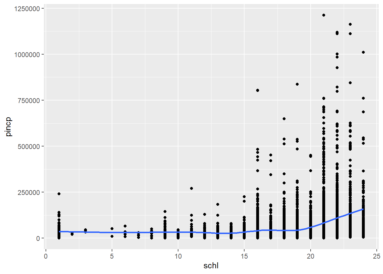

Notice a couple of things. First, the association is much steeper when the average income is higher (or at high levels of schooling). Second, the spread of income is much higher when the average income is high. Both of these issues, non-linearity and heteroscedasticity, might be improved by a log transformation which would compress the extremely high values of income and spread out the low values.

Log transformation

Based on these observations, and on the fact that income is almost always log transformed, I’m going to log transform the income variable. The base is irrelevant, so I’m going to use base 2, just because that’s what I typically use.

acs$l2inc <- log(acs$pincp, base = 2)
acs %>% ggplot(aes(x = schl, y = l2inc)) + geom_point() + geom_smooth(se = FALSE, method = 'loess')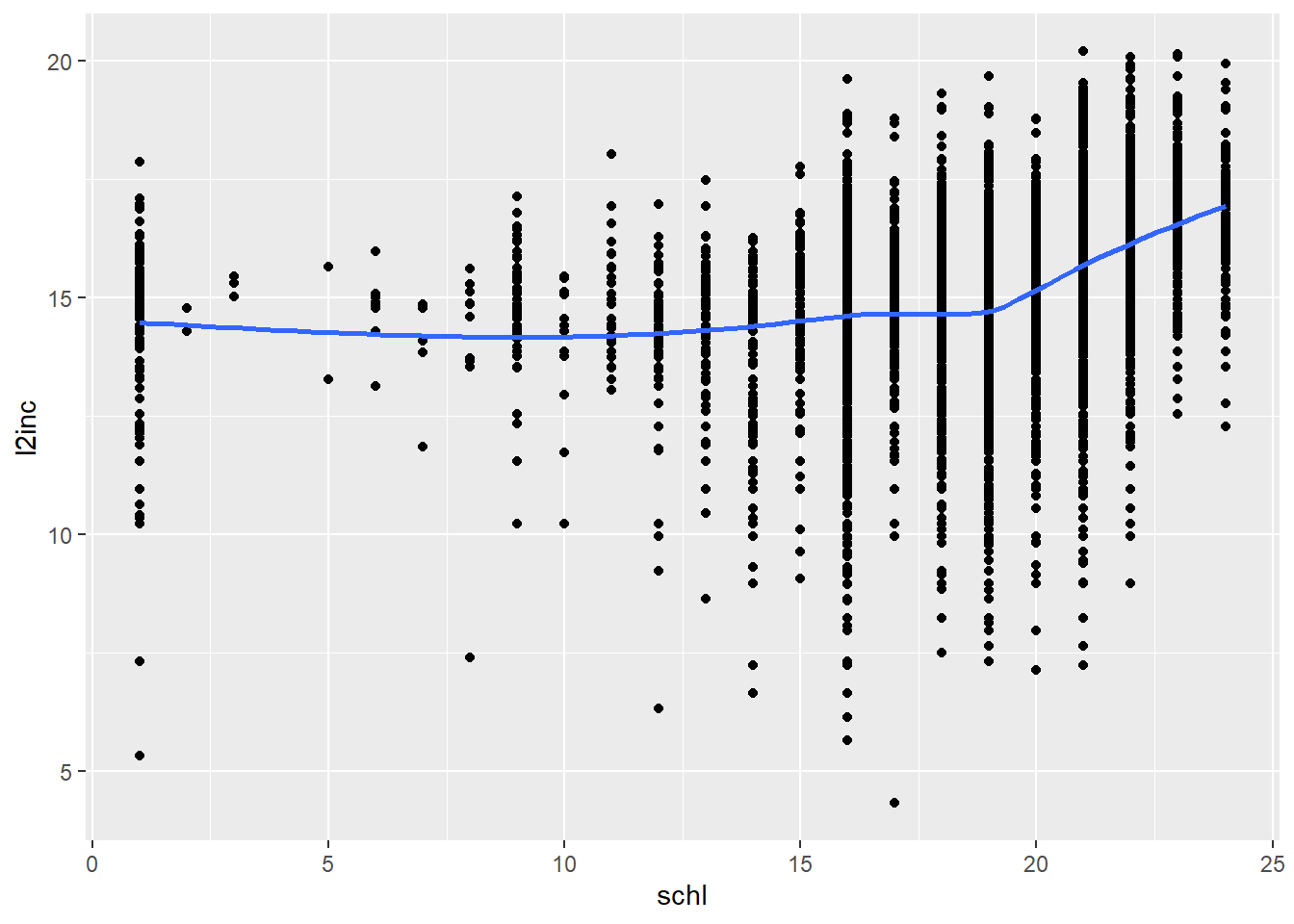

Looking at the scatterplot, I’m honestly not convinced that it’s fixed all of the issues. Heteroscedasticity is much less of an issue, but there’s still some non-linearity (the slope looks a little steeper at high values of education). One reason for this could be that getting a college degree counts a lot more than some of the lower educational levels. However, I’m going to continue with this as though it worked because I want to practice using log transformations and because I genuinely think things look better now.

The Model

The model I’m going to fit it

\log_2(income_i)=\beta_0 + \beta_1schl_i + \varepsilon_i.

library(texreg)
mod <- acs %>% lm(l2inc ~ schl, .)
htmlreg(mod)

Statistical models

	Model 1
(Intercept)	12.44***
	(0.09)
schl	0.15***
	(0.00)
R2	0.09
Adj. R2	0.09
Num. obs.	9998
***p < 0.001; **p < 0.01; *p < 0.05

confint(mod)

             2.5 %     97.5 %

(Intercept) 12.2683093 12.6178123 schl 0.1386774 0.1570372

When we fit this model, we obtain

\hat{\log_2(income_i)} = 12.44 + 0.15schl_i

From the intercept, we estimate that the mean person with a value of 0 for schooling (which is lower than the scale goes) will have an income of about 2^12.44 = \$5,557. We also estimate that each additional level of schooling is associated with a roughly (2^{0.15} - 1)\times100\% = 11\% difference in income. If we were to give this a causal interpretation, which we should not, this would mean that increasing schooling by one level (roughly one additional year of schooling) would increase income by roughly 11%. This association is statistically significant (t(df = 9,996) = 31.6, p < .001), meaning that we have convincing evidence that the association is different from 0 in the population. We’re 95% confident that each level difference in schooling is associated with anywhere between a 10% and and 11.5% difference in schooling. The model explains about 9% of the variation in income, which is a fair amount for something measured at the individual level.

Limitations

In addition to reporting what we found, we want to be clear on what we haven’t found. This is useful both for our audience and for our own understanding.

I’ve mostly discussed these in the unit 5 worked example. I’ll add two things. First, we still can’t be certain that the model is correct. It’s clear that higher education predicts higher income, but it’s not clear that our logarithmic model is correct. In particular, based on the scatterplot, it looks like additional education predicts larger income differences at high levels of education than it does at low levels. Second, we did have restrict our sample by dropping two individuals, so we should be clear that this model on represents American adults who have a positive income.

What’s next?

What’s missing from this analysis? What else would you like to learn about? Send an e-mail to joseph_mcintyre@gse.harvard.edu if you have questions or suggestions!